Just How Live Are Live Query Plans In SQL Server?

Driven to Abstraction


Query plans are generally amusing things in SQL Server.

They aggregate huge amounts of information (in XML!), and then draw it up into a pretty picture that we make a living trying to understand.

Live query plans show you what your query is doing while it’s running.

Sort of.

They don’t show blocking.

Hidden Run


They also don’t show spills. Say I’ve got a query running, and it’s taking a long time.

I’ve got live query plans turned on, so I can see what it’s up to.

A SQL Server query plan
21 minute salute

Hm. Well, that’s not a very full picture. What if I go get the live query plan XML myself?

SELECT deqs.query_plan
FROM sys.dm_exec_sessions AS des
CROSS APPLY sys.dm_exec_query_statistics_xml(des.session_id) AS deqs;

There are three operators showing spills so far.

A SQL Server query plan
Leading me on

Frosted Tips


Even if I go look at the tool tips for operators registering spills, they don’t show anything.

A SQL Server query plan
Do not serve this operator

It’s fine if SSMS doesn’t decide to re-draw icons with little exclamation points, but if information about runtime and rows processed can be updated in real-ish time, information about spills should be, too.

Thanks for reading!

Going Further


If this is the kind of SQL Server stuff you love learning about, you’ll love my training. Blog readers get 25% off the Everything Bundle — over 100 hours of performance tuning content. Need hands-on help? I offer consulting engagements from targeted investigations to ongoing retainers. Want a quick sanity check before committing to a full engagement? Schedule a call — no commitment required.

SQL Server Indexes Sort Data For Us

Yelling and Screaming2019 01 21 13 03 05


If you saw my post about parameterized TOPs, one thing you may have immediately hated is the index I created.

And rightfully so — it was a terrible index for reasons we’ll discuss in this post.

If that index made you mad, congratulations, you’re a smart cookie.

CREATE INDEX whatever ON dbo.Votes(CreationDate DESC, VoteTypeId)
GO

Yes, my friends, this index is wrong.

It’s not just wrong because we’ve got the column we’re filtering on second, but because there’s no reason for it to be second.

Nothing in our query lends itself to this particular indexing scenrio.

CREATE OR ALTER PROCEDURE dbo.top_sniffer (@top INT, @vtid INT)
AS
BEGIN

    SELECT   TOP (@top) 
             v.Id, 
             v.PostId, 
             v.UserId, 
             v.BountyAmount, 
             v.VoteTypeId, 
             v.CreationDate
    FROM     dbo.Votes AS v
    WHERE    v.VoteTypeId = @vtid
    ORDER BY v.CreationDate DESC;

END;

We Index Pretty


The reason I sometimes see columns appear first in an index is to avoid having to physically sort data.

If I run the stored procedure without any nonclustered indexes, this is our query plan:

EXEC dbo.top_sniffer @top = 1, @vtid = 1;
A SQL Server query plan
spillo

A sort, a spill, kablooey. We’re not having any fun, here.

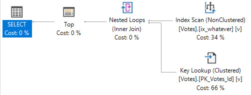
With the original index, our data is organized in the order that we’re asking for it to be returned in the ORDER BY.

This caused all sorts of issues when we were looking for VoteTypeIds that were spread throughout the index, where we couldn’t satisfy the TOP quickly.

There was no Sort in the plan when we had the “wrong” index added.

A SQL Server query plan
Primal

B-Tree Equality


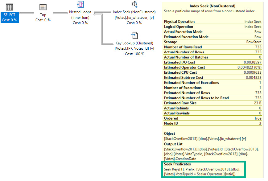
We can also avoid having to sort data by having the ORDER BY column(s) second in the key of the index, because our filter is an equality.

CREATE INDEX whatever ON dbo.Votes(VoteTypeId, CreationDate DESC)
GO

Having the filter column first also helps us avoid the longer running query issue when we look for VoteTypeId 4.

EXEC dbo.top_sniffer @top = 5000, @vtid = 4;
A SQL Server query plan
I like you better.
Table 'Votes'. Scan count 1, logical reads 2262

 SQL Server Execution Times:
   CPU time = 0 ms,  elapsed time = 148 ms.

Solving for Sorts


If you’ve been following my blogging for a while, you’ve likely seen me say this stuff before, because Sorts have some issues.

  • They’re locally blocking, in that every row has to arrive before they can run
  • They require additional memory space to order data the way you want
  • They may spill to disk if they don’t get enough memory
  • They may ask for quite a bit of extra memory if estimations are incorrect
  • They may end up in a query plan even when you don’t explicitly ask for them

There are plenty of times when these things aren’t problems, but it’s good to know when they are, or when they might turn into a problem.

Thanks for reading!

Going Further


If this is the kind of SQL Server stuff you love learning about, you’ll love my training. Blog readers get 25% off the Everything Bundle — over 100 hours of performance tuning content. Need hands-on help? I offer consulting engagements from targeted investigations to ongoing retainers. Want a quick sanity check before committing to a full engagement? Schedule a call — no commitment required.

In SQL Server Stored Procedures, Parameters In TOP Are Sniffed Too

Thank You For Your Business


In yesterday’s post, we looked at how row goals affected performance when data matching our join and where clauses didn’t exist.

Today we’re going to look at something similar, and perhaps a workaround to avoid the same issues.

Here’s our index setup:

CREATE INDEX whatever ON dbo.Votes(CreationDate DESC, VoteTypeId)
GO

Now we’re gonna wrap our query in a stored procedure.

CREATE OR ALTER PROCEDURE dbo.top_sniffer (@top INT, @vtid INT)
AS
BEGIN

    SELECT   TOP (@top) v.*
    FROM     dbo.Votes AS v
    WHERE    v.VoteTypeId = @vtid
    ORDER BY v.CreationDate DESC;

END;

Video Killed MTV


You know what? I don’t wanna write all this stuff. Let’s do a video.

Thanks for reading!

Video Summary

In this video, I dive into an interesting scenario involving parameterized `TOP` in SQL Server stored procedures. I explore how SQL Server handles rare data searches and the impact on query performance when using parameters like `TOP`. By creating a specific index and running various queries, I demonstrate how SQL Server’s caching mechanism can lead to suboptimal plans for rare data lookups, showcasing both the challenges and potential solutions. I also touch on some lesser-known behaviors, such as the parameter sniffing issues that arise with `OPTIMIZE FOR UNKNOWN` and dynamic SQL alternatives, providing insights into optimizing your stored procedures for better performance in real-world scenarios.

Full Transcript

Howdy folks, Erik Darling here with, well, with Erik Darling Data. And I wanted to record this as a video because I am far too lazy to blog about this today. It’s Sunday and I don’t want to do all that work screen capping and highlighting stuff and all that other things that go along with a great post. So I’m just going to record this video because I think that’s going to be a little bit easier on everyone. So what I got is something kind of funny to show you about what happens when we parameterize top. In other words, when we write a query, a stored procedure, or whatever you want to call it, and we allow people to pass a parameter like this to top like this. Now, I found some interesting stuff in this. Hopefully you find it interesting too. Now I’ve got an index here. You can ignore that little red squiggle. It’s because I already created it ahead of time because I know how much everyone hates waiting for indexes to create. And it’s on creation date descending and vote type ID. Now that is there mostly to satisfy this part of the query, my where clause on vote type ID and my order by on creation date. I know that for a bunch of the columns I’m selecting here, I’m going to have to do a key lookup. That’s not really what this is about. What I want to show you is what happens when SQL Server has to go looking for rare data. Now in the votes table, the way things break down is there are kind of a lot of rows with a vote type ID of one. There are about 3.7 million. There are far fewer with a vote type ID of four. There’s only about 733. The way that they break down in the index is fairly even. So when we look at the year of the creation date, remember that’s the leading column in the index. Oops, jumped around a little bit there. We can see that things break down fairly evenly across all of the possible years here. There’s not like any great big gaps. We have one in just about every year in the index. Everything’s pretty even there. Now when we run the plan, I’m just going to recompile this thing real quick to make sure I’m getting something fresh out the bag. And I look for the top 5,000 rows for vote type ID one. This runs fairly quickly. This runs in around about 23 milliseconds total. And it does about 15,000 logical reads. So that’s good.

And when we look at the execution plan. What I want to show you first is that when we look at the parameters that got passed in, top just like any other parameter was cached. So we have a parameter compile value of 5,000. And we also have a parameter runtime value of 5,000. If I get rid of this, and we go look at an execution where we have a 1 in as top, exactly what you think is going to happen happens. We hit F4. We go look at the plan properties. Got to jump around a little bit to get to the right one. And when I look at the parameter list. Now I have a compile time value of 5,000. And a runtime value of 1. So just like any other parameter in a store procedure in SQL Server, it gets cached when we run the query the first time.

And then it gets reused when we run the query subsequent times. Now, obviously, this could backfire if we recompile here, and we run the plan looking for a top one first. And then the next execution, some ding dong comes along and looks for a million rows. This is the obvious one. We’re going to reuse that tiny little plan that SQL Server came up with to find one row, and we’re going to use it to find a million rows. That’s the obvious bad part of parameter sniffing. The kind of less bad part, or the kind of more interesting bad part, is what happens when we look for data that is a little bit harder to find, that rare data. So now I’m going to look for a top one for the vote type ID of 4. Remember, this is the one that only has about 773 rows in the table. But when I look for top one, it’s fast.

Because it finds a row really early in the index that it can give back. Again, this is going to be early in the index, it’s order descending. So it finds this row from 2013 and says, good, we’re done. If I say I want the top 5,000 where vote type ID equals 4, this is going to be a little bit less snappy. Now we’re going to spend about two seconds, or actually close to three seconds, scanning the entire index and looking for data.

You can see that we spent an elapsed 2,700 milliseconds, close enough to three seconds for me. And we did, let’s see, that’s 146,534 reads. So we had to scan that entire index looking for that kind of spread out, kind of rare vote type ID for.

We had to start at the beginning, which is going to be the year 2013. And we had to go all the way to the end, which is 2008. So that’s one example.

Now what’s kind of interesting that I found is if I recompile things, if I clear out the plan for that store procedure, and I look for the top 5,000 first. Now even though I know that 5,000 rows don’t exist, that’s not really an issue here because the top will exit when the nested loops join says, I don’t have any more rows to give you. The top says, okay, well I wanted 5,000, thanks a lot.

So if we run this first, the plan changes a little. And it changes in that it goes parallel now. SQL Server says, I think I might have to spend a little bit more time reading this. I’m actually going to go parallel.

I’m going to use multiple threads to find these rows because they’re spread out everywhere. So that’s kind of a cool thing that SQL Server knew to do. And then when I rerun, of course, looking for a top 1, it’s going to reuse that parallel plan. And things are going to be fairly snappy still, right? It’s still okay. We’re still running in under a sec.

We’re still pretty well under a second there. Now, something else interesting that I came across when I was messing with stuff is that if you use optimize for unknown and you use a variable for top, you get kind of a funky guess just like you do with most other unknown guesses. Now, what I’ve done for this run of the store procedure is I’ve quoted out the vote type ID part of the where clause because I don’t want you thinking that the row estimate is coming from the vote type ID that I’ve chosen to pass in.

That’s not where it’s coming from. If I recompile the query without that where clause in it, and just for good luck, I’m going to make sure it’s extra double recompiled. I’m going to run this now looking for the top 5,000 rows.

And when I go look at the execution plan, rather than guessing 5,000, my top has a guess of 100. So when you use optimize for unknown with a parameterized top, you always get this guess of 100. I tried lots of different numbers, and the only time that it was never not 100 is if I recompile it through a recompile hint on that.

So that was a little funny. Anyway, if you use top in a parameterized sort of way, there are some things you might want to explore if you’re running into problems. If you’re recompiling the plan, if unparameterized or even non-parameterized, dynamic SQL might help.

Now, I say that, and I know people are going to crawl out of their skin because unparameterized dynamic SQL can lead to SQL injection attacks. I know that it’s a lesson to a degree because you would be using an integer with top, and likely just using a function like rtrim or something to produce a stringified version of the number to concatenate into the query.

But the risk is still there, so be careful. You might want to say, okay, if I know that under certain conditions I want a different plan for things, do I need to separate code into different store procedures?

Or do I have an optimized for a value? Like if I, rather than doing optimized for unknown, can I optimize for a value like 5,000, 10,000, 2.1 billion, whatever Adam Mechanics phone number is, and get a better plan that way? Do I need to change indexes?

Like maybe the order of the key of the index has been appropriate for the query? Do I need to have some included columns to get rid of that key lookup? Do I need to make an adjustment there? So there’s a lot of stuff that you could look at as ways to solve it, but this is just to let you know that that issue exists, and maybe if you keep reading my blog posts and stuff like that, maybe we’ll talk about all the ways that you can fix it coming up.

Anyway, I hope you enjoyed yourselves. I hope you learned some stuff. I mean, who knows? Maybe you didn’t. If you’re smart, you didn’t learn anything. I hope you were at least entertained if you didn’t learn anything. Anyway, I am Erik Darling with Erik Darling Data, and thanks for watching.

Bye.

Going Further


If this is the kind of SQL Server stuff you love learning about, you’ll love my training. Blog readers get 25% off the Everything Bundle — over 100 hours of performance tuning content. Need hands-on help? I offer consulting engagements from targeted investigations to ongoing retainers. Want a quick sanity check before committing to a full engagement? Schedule a call — no commitment required.

SQL Server Query Performance When You Search For Rare Data Points

I Got No Rows


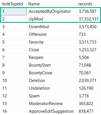
Over in the Votes table in the Stack Overflow database, a couple of the more popular vote types are 1 and 2.

A vote type of 1 means that an answer was accepted as being the solution by a user, and a vote type of 2 means someone upvoted a question or answer.

SQL Server Query Results
I Voted!

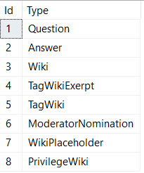
What this means is that it’s impossible for a question to ever have an accepted answer vote cast for it. A question can’t be an answer, here.

Unfortunately, SQL Server doesn’t have a way of inferring that.

SQL Server Query Results
ANSWER ME!

Anything with a post type id of 1 is a question.

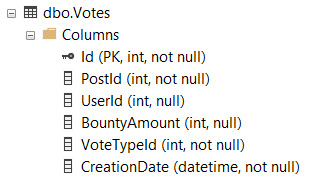
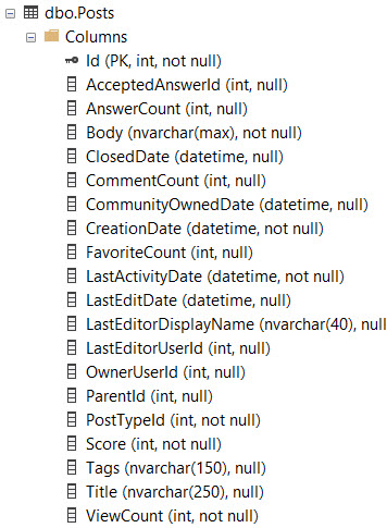
The way the tables are structured, VoteTypeId and PostTypeId don’t exist together, so we can’t use a constraint to validate any conditions that exist between them.

SQL Server Management Studio Table
Votan
SQL Server Management Studio Table
Postan

Lost And Found


When we run a query that looks for posts with a type of 2 (that’s an answer) that have a vote type of 1, we can find 2500 of them relatively quickly.

    SELECT   TOP (2500) 
             p.OwnerUserId, 
             p.Score, 
             p.Title, 
             v.CreationDate,
             ISNULL(v.BountyAmount, 0) AS BountyAmount
    FROM     dbo.Posts AS p
    JOIN     dbo.Votes AS v
        ON  p.Id = v.PostId
    WHERE v.VoteTypeId = 2 --WHERE VoteTypeId = 2
    AND   p.PostTypeId = 1
    ORDER BY v.CreationDate DESC;

Here’s the stats:

Table 'Posts'. Scan count 0, logical reads 29044
Table 'Votes'. Scan count 1, logical reads 29131

 SQL Server Execution Times:
   CPU time = 63 ms,  elapsed time = 272 ms.

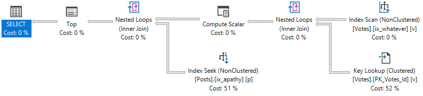
And here’s the plan:

SQL Server Query Plan
Nelly.

Colossus of Woes


Now let’s ask SQL Server for some data that doesn’t exist.

    SELECT   TOP (2500) 
             p.OwnerUserId, 
             p.Score, 
             p.Title, 
             v.CreationDate,
             ISNULL(v.BountyAmount, 0) AS BountyAmount
    FROM     dbo.Posts AS p
    JOIN     dbo.Votes AS v
        ON  p.Id = v.PostId
    WHERE v.VoteTypeId = 1 --Where VoteTypeId = 1
    AND   p.PostTypeId = 1
    ORDER BY v.CreationDate DESC;

Here’s the stats:

Table 'Posts'. Scan count 0, logical reads 11504587
Table 'Votes'. Scan count 1, logical reads 11675392

 SQL Server Execution Times:
   CPU time = 14813 ms,  elapsed time = 14906 ms.

You could say things got “worse”.

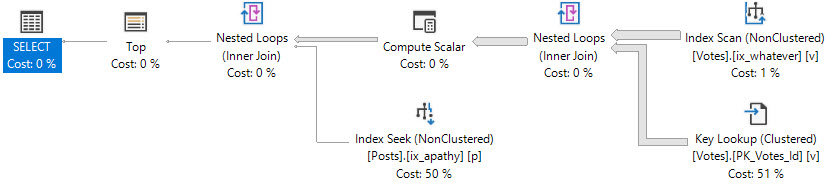
Not only that, but they got worse for the exact same plan.

SQL Server Query Plan
Argh.

So What Happened?


In the original plan, the TOP asked for rows, and quickly got them.

In the second plan, the TOP kept asking for rows, getting them from the Votes table, and then losing them on the join to Posts.

There was no parameter sniffing, there were no out of date stats, no blocking, or any other oddities. It’s just plain bad luck because of the data’s relationship.

If we apply hints to this query to:

  • Scan the clustered index on Votes
  • Choose Merge or Hash joins instead of Nested Loops
  • Force the join order as written

We get much better performing queries. The plan we have is chosen because the TOP sets a row goal that makes a Nested Loops plan using narrow (though not covering) indexes attractive to the optimizer. When it’s right, like in the original query, you probably don’t even think about it.

When it’s wrong, like in the second query, it can be quite mystifying why such a tiny query can run forever to return nothing.

If you want to try it out for yourself, use these indexes:

    CREATE INDEX whatever 
        ON dbo.Votes( CreationDate, VoteTypeId, PostId );

    CREATE NONCLUSTERED INDEX apathy
        ON dbo.Posts ( PostTypeId )
            INCLUDE ( OwnerUserId, Score, Title );

Thanks for reading!

Going Further


If this is the kind of SQL Server stuff you love learning about, you’ll love my training. Blog readers get 25% off the Everything Bundle — over 100 hours of performance tuning content. Need hands-on help? I offer consulting engagements from targeted investigations to ongoing retainers. Want a quick sanity check before committing to a full engagement? Schedule a call — no commitment required.

The Resource Governor MAXDOP Setting Can Lead to Poor Plan Choices In SQL Server

Resource Governor can be used to enforce a hard cap on query MAXDOP, unlike the sp_configure setting. However, query plan compilation does not take such a MAXDOP limit into account. As a result, limiting MAXDOP through Resource Governor can lead to unexpected degradations in performance due to suboptimal query plan choices.

Create Your Tables


We start with the not often seen here three table demo. I’d rather not explain how I came up with this sample data, so I’m not going to. I did my testing on a server with max server memory set to 10000 MB. The following tables take about half a minute to create and populate and only take up about 1.5 GB of space:

DROP TABLE IF EXISTS dbo.SMALL;
CREATE TABLE dbo.SMALL (ID_U NUMERIC(18, 0));

INSERT INTO dbo.SMALL WITH (TABLOCK)
SELECT TOP (100) 5 * ROW_NUMBER()
	OVER (ORDER BY (SELECT NULL))
FROM master..spt_values t1
CROSS JOIN master..spt_values t2
OPTION (MAXDOP 1);

DROP TABLE IF EXISTS dbo.MEDIUM;
CREATE TABLE dbo.MEDIUM (ID_A NUMERIC(18, 0));

INSERT INTO dbo.MEDIUM WITH (TABLOCK)
SELECT TOP (600000) ROW_NUMBER()
	OVER (ORDER BY (SELECT NULL))
FROM master..spt_values t1
CROSS JOIN master..spt_values t2
CROSS JOIN master..spt_values t3
OPTION (MAXDOP 1);

DROP TABLE IF EXISTS dbo.LARGE;
CREATE TABLE dbo.LARGE (
	ID_A NUMERIC(18, 0),
	ID_U NUMERIC(18, 0),
	FILLER VARCHAR(100)
);

INSERT INTO dbo.LARGE WITH (TABLOCK)
SELECT 2 * ( RN / 4), RN % 500, REPLICATE('Z', 100)
FROM
(
	SELECT TOP (8000000) ROW_NUMBER()
		OVER (ORDER BY (SELECT NULL)) RN
	FROM master..spt_values t1
	CROSS JOIN master..spt_values t2
	CROSS JOIN master..spt_values t3
) q
OPTION (MAXDOP 1)

CREATE INDEX IA ON LARGE (ID_A);
CREATE INDEX IU ON LARGE (ID_U);

The Long-Awaited Demo


I thought up the theory behind this demo on a car ride back from a SQL Saturday, but wasn’t able to immediately figure out a way to get the query plan that I wanted. I ended up finally seeing it in a totally different context and am now happy to share it with you. Consider the following query:

SELECT LARGE.ID_U
FROM dbo.SMALL
INNER JOIN dbo.LARGE ON SMALL.ID_U = LARGE.ID_U
INNER JOIN dbo.MEDIUM ON LARGE.ID_A = MEDIUM.ID_A
OPTION (MAXDOP 1);

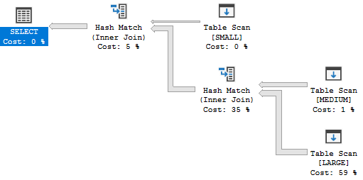
The MAXDOP 1 hints results in a serial plan with two hash joins:

a36_MAXDOP1_plan

This is a perfectly reasonable plan given the size and structure of the tables. There are no bitmap filters because row mode bitmap filters are only supported for parallel plans. Batch mode is not considered for this query because I’m testing on SQL Server 2017 and there isn’t a columnstore index on any of the tables referenced in the query. On my machine a single query execution uses 2422 of CPU time and 2431 ms of elapsed time.

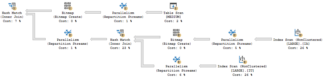
A parallel plan at MAXDOP 4 is able to run more quickly but with a much higher CPU time. A single execution of the MAXDOP 4 query uses 5875 ms of CPU time and 1617 ms of elapsed time. There are multiple bitmap filters present. I zoomed in on the most interesting part of the plan because I haven’t figured out how images work with WordPress yet:

a36_MAXDOP4_plan

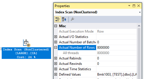
Instead of doing a scan of the LARGE table, SQL Server instead chooses an index intersection plan. The cost of the additional hash join is reduced by multiple bitmap filters. There are only 2648396 and 891852 rows processed on the build and probe side instead of 8 million for each side, which is a significant gain.

Worse Than A Teen Running for Governor


Some end users really can’t be trusted with the power to run parallel plans. I thought about making a joke about an “erik” end user but I would never subject my readers to the same joke twice. After enforcing a MAXDOP of 1 at the Resource Governor level, you will probably not be shocked to learn that the query with the explicit MAXDOP 1 hint gets the same query plan as before and runs with the same amount of CPU and elapsed time.

If you skipped or forget the opening paragraph, you may be surprised to learn that the query with a MAXDOP 4 hint also gets the same query plan as before. The actual execution plan even has the parallel racing arrows. However, the query cannot execute in parallel. The parallelism and bitmap operators are skipped by the query processor and all of the rows are processed on one thread:

a36_MAXDOP4_with_RG

I uploaded the query plan here if you want to look at it. This type of scenario can happen even without Resource Governor. For example, a compiled parallel query may be downgraded all the way to MAXDOP 1 if it can’t get enough parallel threads.

The query performs significantly worse than before, which hopefully is not a surprise. A single execution took 12860 ms of CPU time and 13078 ms of elapsed time. Nearly all of the query’s time is spent on the hash join for the index intersection, with a tempdb spill and the processing of additional rows both playing a role. The tempdb spill occurs because SQL Server expected the build side of the hash join to be reduced to 1213170 rows. The bitmap filtering does not occur so 8 million rows were sent to the build side instead.

In this case, adding a MAXDOP 1 hint to the query will improve performance by about 5X. Larger differences in run times can be easily seen on servers with more memory than my desktop.

Final Thoughts


If you’re using using Resource Governor to limit MAXDOP to 1, consider adding explicit MAXDOP 1 hints at the query level if you truly need the best possible performance. The MAXDOP 1 hint may at first appear to be redundant, but it gives the query optimizer additional information which can result in totally different, and sometimes significantly more efficient, query plans. I expect that this problem could be avoided if query plan caching worked on a Resource Governor workload group level. Perhaps that is one of those ideas that sounds simple on paper but would be difficult for Microsoft to implement. Batch mode for row store can somewhat mitigate this problem because batch mode bitmap filters operate even under MAXDOP 1, but you can still get classic row mode bitmaps even on SQL Server 2019.

Thanks for reading!

Going Further


If this is the kind of SQL Server stuff you love learning about, you’ll love my training. Blog readers get 25% off the Everything Bundle — over 100 hours of performance tuning content. Need hands-on help? I offer consulting engagements from targeted investigations to ongoing retainers. Want a quick sanity check before committing to a full engagement? Schedule a call — no commitment required.

A Row Goal Riddle In SQL Server

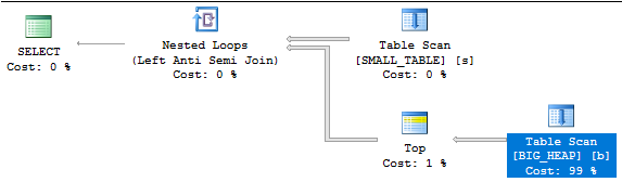
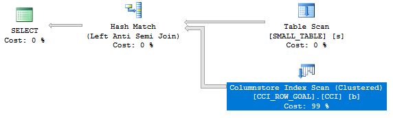
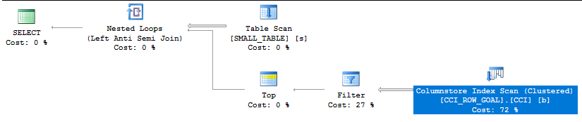
I’m the kind of guy who sometimes likes to look at execution plans with different hints applied to see how the plan shape and query operator costs change. Sometimes paying attention to operator costs can provide valuable clues as to why the query optimizer selected a plan that you didn’t like. Sometimes it doesn’t. My least favorite scenario is when I see inconsistent operator costs. This blog post covers a reproduction of such a case involving the dreaded and feared row goal.

The Data


For the data in my demo tables, I wanted a query of the following form:

SELECT *FROM dbo.OUTER_HEAP oWHERE NOT EXISTS(SELECT 1FROM dbo.INNER_CI iWHERE i.ID = o.ID);

that returned zero rows. However, I wanted the query optimizer to think that a decent number of rows would be returned. This was more difficult to do than expected. I could have just hacked stats to easily accomplish what I wanted, but did not do so out of stubbornness and pride. I eventually found a data set through trial and error with a final cardinality estimate of 16935.2 rows, or 1.7% of the rows in the outer table:

DROP TABLE IF EXISTS dbo.OUTER_HEAP;CREATE TABLE dbo.OUTER_HEAP (ID VARCHAR(10));INSERT INTO dbo.OUTER_HEAP WITH (TABLOCK)SELECT TOP (1000000) 1500000+ ROW_NUMBER() OVER (ORDER BY (SELECT NULL))FROM master..spt_values t1CROSS JOIN master..spt_values t2OPTION (MAXDOP 1);CREATE STATISTICS S1 ON dbo.OUTER_HEAP (ID)WITH FULLSCAN;DROP TABLE IF EXISTS dbo.INNER_CI;CREATE TABLE dbo.INNER_CI (ID VARCHAR(10),PRIMARY KEY (ID));INSERT INTO dbo.INNER_CI WITH (TABLOCK)SELECT TOP (2000000) 500000+ ROW_NUMBER() OVER (ORDER BY (SELECT NULL))FROM master..spt_values t1CROSS JOIN master..spt_values t2OPTION (MAXDOP 1);CREATE STATISTICS S1 ON dbo.INNER_CI (ID)WITH FULLSCAN;

The actual query of interest is the following one:

SELECT TOP (1) 1FROM dbo.OUTER_HEAP oWHERE NOT EXISTS(SELECT 1FROM dbo.INNER_CI iWHERE i.ID = o.ID);

Such a query might be used as part of an ETL process as some kind of data validation step. The most interesting case to me is when the query returns no rows, but the query optimizer (for whatever reason) thinks otherwise.

Row Goal Problems


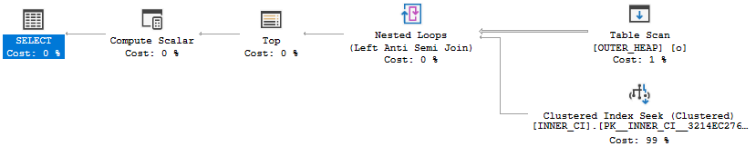
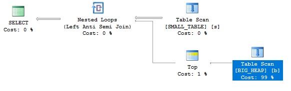
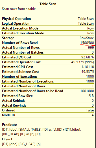
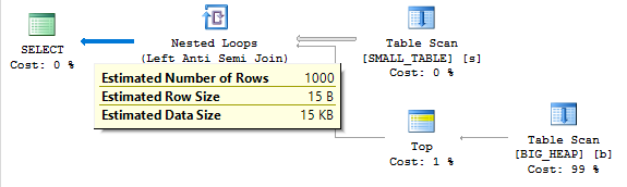
On my machine I get the following plan for the TOP (1) query:a29_row_goal_nlThe plan has a total cost of 0.198516 optimizer units. If you know anything about row goals (this may be a good time for the reader to visit Paul White’s series on row goals) you might not be terribly surprised by the outcome. The row goal introduced by the TOP (1) makes the nested loop join very attractive in comparison to other plan choices. The cost of the scan on OUTER_HEAP is discounted from 2.93662 units to 0.0036173 units and the optimizer only expects to do 116 clustered index seeks against INNER_CI before it finds a row that does not match. However, we know our data and we know that all rows match. Therefore, the query will not return any rows and it must scan all rows in OUTER_HEAP if I execute the query. On my machine the query takes about two seconds:

CPU time = 1953 ms, elapsed time = 1963 ms.

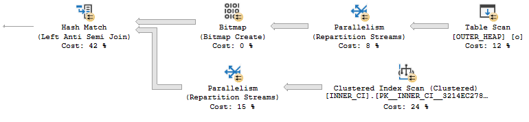
If we’re going to read most of the rows anyway why not try a HASH JOIN hint? At least that plan won’t have a million clustered index seeks:a29_HJ_PLANThe new plan runs in MAXDOP 4 on my machine (although for not very long due to CPU cooling issues) and has a total cost of 19.9924 optimizer units. Query execution finishes in significantly less time:

CPU time = 1187 ms, elapsed time = 372 ms.

The Riddle


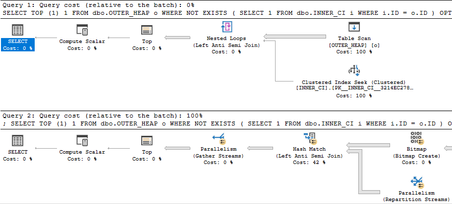
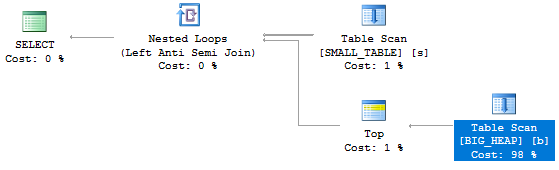
Can we do better than an ugly join hint? Microsoft blessed us with USE HINT functionality in SQL Server 2016 SP1, so let’s go ahead and try that to see if we can improve the performance of the query. To understand the full effect of the hint let’s get estimated plans for OPTION clauses of (USE HINT ('DISABLE_OPTIMIZER_ROWGOAL'), LOOP JOIN) and (USE HINT ('DISABLE_OPTIMIZER_ROWGOAL'), HASH JOIN). In theory, that will make it easy to compare the two queries:a29_compare_plansSomething looks very wrong here. The loop join plan has a significantly lower cost than the hash join plan! In fact, the loop join plan has a total cost of 0.0167621 optimizer units. Why would disabling row goals for such a plan cause a decrease in total query cost?I uploaded the estimated plans here for those who wish to examine them without going through the trouble of creating tables.

Let’s Try Adding Trace Flags


First let’s try the query with just a USE HINT and no join hint. I get the hash join plan shape that I was after with a total cost of 19.9924 optimizer units. That’s definitely a good thing, but why did the optimizer pick that plan? The plan with a loop join is quite a bargain at 0.0167621 optimizer units. The optimization level is FULL, but that doesn’t mean that every possible plan choice was evaluated. Perhaps the answer is as simple as the optimizer did not consider a nested loop join plan while evaluating possible plan choices.There are a few different ways to see which optimizer rules were considered during query plan compilation. We can add trace flags 3604 and 8619 at the query level to get information about the rules that were applied during optimization. All of these trace flags are undocumented, don’t use them in production, blah blah blah. For clarity, the query now looks like this:

SELECT TOP (1) 1FROM dbo.OUTER_HEAP oWHERE NOT EXISTS(SELECT 1FROM dbo.INNER_CI iWHERE i.ID = o.ID) OPTION (USE HINT ('DISABLE_OPTIMIZER_ROWGOAL'), QUERYTRACEON 3604, QUERYTRACEON 8619);

Among other rules, we can see a few associated with nested loops:Apply Rule: LeftSideJNtoIdxLookup - LOJN/LSJ/LASJ -> IDX LOOKUPApply Rule: LASJNtoNL - LASJN -> NL

So the optimizer did consider nested loop joins at some point but it went with the hash join plan instead. That's interesting.

Let's Try More Trace Flags


A logical next step is to try to get more operator costing information. Perhaps the cost of the nested loop join plan when considered during optimization is different from the value displayed in the query plan in SSMS. As the optimizer applies different rules and does different transformations the overall cost can change, so I suppose this isn't a totally unreasonable theory. My first attempt at getting cost information for multiple plan options is by looking at the final memo for the query. This can be done with trace flag 8615.For clarity, the query now looks like this:

SELECT TOP (1) 1FROM dbo.OUTER_HEAP oWHERE NOT EXISTS(SELECT 1FROM dbo.INNER_CI iWHERE i.ID = o.ID) OPTION (USE HINT ('DISABLE_OPTIMIZER_ROWGOAL'), QUERYTRACEON 3604, QUERYTRACEON 8615-- , QUERYTRACEON 8619);

Group 8 is the only one with any costing information for joins:Group 8: Card=16935.2 (Max=1.1e+006, Min=0)11 PhyOp_HashJoinx_jtLeftAntiSemiJoin 6.9 7.10 5.0 Cost(RowGoal 0,ReW 0,ReB 0,Dist 0,Total 0)= 26.5569 (Distance = 1)4 PhyOp_HashJoinx_jtLeftAntiSemiJoin 6.4 7.3 5.0 Cost(RowGoal 0,ReW 0,ReB 0,Dist 0,Total 0)= 38.4812 (Distance = 1)1 LogOp_RightAntiSemiJoin 7 6 5 (Distance = 1)0 LogOp_LeftAntiSemiJoin 6 7 5 (Distance = 0)

This is rather disappointing. There's only costing information for a few hash join plans. We know that other join types were considered. Perhaps they were discarded from the memo. The final memo just doesn't have enough information to answer our question.

We Must Not Be Using Enough Trace Flags


There's a trace flag that adds memo arguments to trace flag 8619: 8620. Perhaps that will give us additional clues. For clarity, the query now looks like this:

SELECT TOP (1) 1FROM dbo.OUTER_HEAP oWHERE NOT EXISTS(SELECT 1FROM dbo.INNER_CI iWHERE i.ID = o.ID) OPTION (USE HINT ('DISABLE_OPTIMIZER_ROWGOAL'), QUERYTRACEON 3604, QUERYTRACEON 8615, QUERYTRACEON 8619, QUERYTRACEON 8620);

The output is again disappointing. I'll skip covering it and jump to trace flag 8621. That one adds additional information about the rules and how they interact with memos. With this trace flag we find more information about the plans with merge or loop joins:Rule Result: group=8 1 LogOp_RightAntiSemiJoin 7 6 5 (Distance = 1)Rule Result: group=8 2 PhyOp_MergeJoin 1-M x_jtRightAntiSemiJoin 7 6 5 (Distance = 2)Rule Result: group=8 3 PhyOp_HashJoinx_jtRightAntiSemiJoin 7 6 5 (Distance = 2)Rule Result: group=8 4 PhyOp_HashJoinx_jtLeftAntiSemiJoin 6 7 5 (Distance = 1)Rule Result: group=8 5 PhyOp_Applyx_jtLeftAntiSemiJoin 6 16 (Distance = 1)Rule Result: group=8 6 PhyOp_Applyx_jtLeftAntiSemiJoin 6 16 (Distance = 1)Rule Result: group=8 7 PhyOp_LoopsJoinx_jtLeftAntiSemiJoin 6 17 5 (Distance = 1)Rule Result: group=8 8 PhyOp_LoopsJoinx_jtLeftAntiSemiJoin 6 7 5 (Distance = 1)Rule Result: group=8 9 PhyOp_MergeJoin 1-M x_jtRightAntiSemiJoin 7 6 5 (Distance = 2)Rule Result: group=8 10 PhyOp_HashJoinx_jtRightAntiSemiJoin 7 6 5 (Distance = 2)Rule Result: group=8 11 PhyOp_HashJoinx_jtLeftAntiSemiJoin 6 7 5 (Distance = 1)Rule Result: group=8 12 PhyOp_Applyx_jtLeftAntiSemiJoin 6 16 (Distance = 1)Rule Result: group=8 13 PhyOp_Applyx_jtLeftAntiSemiJoin 6 16 (Distance = 1)Rule Result: group=8 14 PhyOp_LoopsJoinx_jtLeftAntiSemiJoin 6 17 5 (Distance = 1)Rule Result: group=8 15 PhyOp_LoopsJoinx_jtLeftAntiSemiJoin 6 17 5 (Distance = 1)Rule Result: group=8 16 PhyOp_LoopsJoinx_jtLeftAntiSemiJoin 6 7 5 (Distance = 1)Rule Result: group=8 17 PhyOp_LoopsJoinx_jtLeftAntiSemiJoin 6 7 5 (Distance = 1)

However, group 8 in the final memo still looks the same as before:Group 8: Card=16935.2 (Max=1.1e+006, Min=0)11 PhyOp_HashJoinx_jtLeftAntiSemiJoin 6.9 7.10 5.0 Cost(RowGoal 0,ReW 0,ReB 0,Dist 0,Total 0)= 26.5569 (Distance = 1)4 PhyOp_HashJoinx_jtLeftAntiSemiJoin 6.4 7.3 5.0 Cost(RowGoal 0,ReW 0,ReB 0,Dist 0,Total 0)= 38.4812 (Distance = 1)1 LogOp_RightAntiSemiJoin 7 6 5 (Distance = 1)0 LogOp_LeftAntiSemiJoin 6 7 5 (Distance = 0)

My interpretation is that costing information for the other join types was discarded from the memo. For example, at one point there was an item 5 in group 8 which contained information relevant to costing for one of the nested loop join plans. All of that information is not present in the final plan because the hash join plan was cheaper.

Pray to the Trace Flag Gods


There is an undisclosed trace flag which does not allow items to be discarded from the memo. Obviously this is a dangerous thing to do. However, with that trace flag group 8 finally reveals all of its secrets:Group 8: Card=16935.2 (Max=1.1e+006, Min=0)17 PhyOp_LoopsJoinx_jtLeftAntiSemiJoin 6 7 5.0 (Distance = 1)16 PhyOp_LoopsJoinx_jtLeftAntiSemiJoin 6 7 5.0 (Distance = 1)15 PhyOp_LoopsJoinx_jtLeftAntiSemiJoin 6 17 5.0 (Distance = 1)14 PhyOp_LoopsJoinx_jtLeftAntiSemiJoin 6 17 5.0 (Distance = 1)13 PhyOp_Applyx_jtLeftAntiSemiJoin 6 16 (Distance = 1)12 PhyOp_Applyx_jtLeftAntiSemiJoin 6 16 (Distance = 1)11 PhyOp_HashJoinx_jtLeftAntiSemiJoin 6.9 7.10 5.0 Cost(RowGoal 0,ReW 0,ReB 0,Dist 0,Total 0)= 26.5569 (Distance = 1)10 PhyOp_HashJoinx_jtRightAntiSemiJoin 7.8 6 5 (Distance = 2)9 PhyOp_MergeJoin 1-M x_jtRightAntiSemiJoin 7.6 6 5 (Distance = 2)8 PhyOp_LoopsJoinx_jtLeftAntiSemiJoin 6 7 5.0 (Distance = 1)7 PhyOp_LoopsJoinx_jtLeftAntiSemiJoin 6 17 5.0 (Distance = 1)6 PhyOp_Applyx_jtLeftAntiSemiJoin 6 16 (Distance = 1)5 PhyOp_Applyx_jtLeftAntiSemiJoin 6 16 (Distance = 1)4 PhyOp_HashJoinx_jtLeftAntiSemiJoin 6.4 7.3 5.0 Cost(RowGoal 0,ReW 0,ReB 0,Dist 0,Total 0)= 38.4812 (Distance = 1)3 PhyOp_HashJoinx_jtRightAntiSemiJoin 7.3 6.4 5.0 Cost(RowGoal 0,ReW 0,ReB 0,Dist 0,Total 0)= 48.5597 (Distance = 2)2 PhyOp_MergeJoin 1-M x_jtRightAntiSemiJoin 7.1 6.2 5.0 Cost(RowGoal 0,ReW 0,ReB 0,Dist 0,Total 0)= 106.564 (Distance = 2)1 LogOp_RightAntiSemiJoin 7 6 5 (Distance = 1)0 LogOp_LeftAntiSemiJoin 6 7 5 (Distance = 0)

Let's consider item 5 because it's one of the more reasonable loop join plan options. Item 5 doesn't give us direct costing information but it directs us to look to group 16:Group 16: Card=1 (Max=1, Min=0)2 PhyOp_Range 1 ASC 5.0 Cost(RowGoal 0,ReW 0,ReB 999999,Dist 1e+006,Total 1e+006)= 165.607 (Distance = 2)1 PhyOp_Range 1 ASC 5.0 Cost(RowGoal 0,ReW 0,ReB 999999,Dist 1e+006,Total 1e+006 s)= 165.607 (Distance = 2)0 LogOp_SelectIdx 15 5 (Distance = 1)

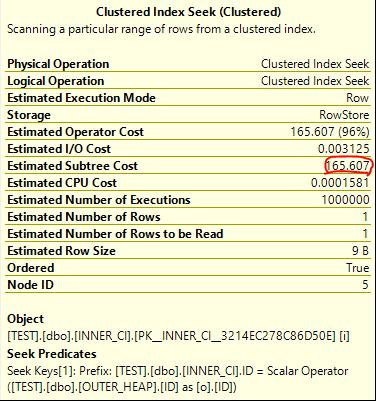
We can see a cost of 165.607 for the clustered index seeks on the inner side of the join. If that was the cost used when comparing plans then it explains why the optimizer opted for a hash join over the loop join. We might try looking at a query plan for the following:

DECLARE @TOP INT = 1;SELECT TOP (@TOP) 1FROM dbo.OUTER_HEAP oWHERE NOT EXISTS(SELECT 1FROM dbo.INNER_CI iWHERE i.ID = o.ID)OPTION (OPTIMIZE FOR (@TOP = 987654321), LOOP JOIN, MAXDOP 1);

With the above syntax we will get the same query results as before but the effective TOP (1) cannot change the cost of the query. Here are the operator details for the clustered index seek on INNER_CI:a29_seek_costsIt's an exact match. The total cost of the query is 172.727 optimizer units, which is significantly more than the price tag of 19.9924 units for the hash join plan.

Improving Displayed Costing


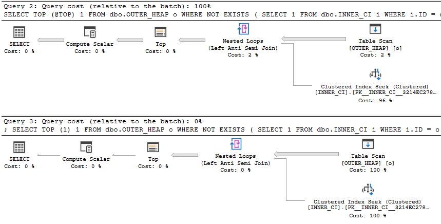
So is there really a problem with the displayed cost of the plan with hints matching (USE HINT ('DISABLE_OPTIMIZER_ROWGOAL'), LOOP JOIN)? After all, the USE HINT seemed to give the correct plan shape without the join hints. Let's compare the TOP plan side by side with it:a29_compare_nl_plansI also uploaded the estimated plans here.In my view, the costs of the USE HINT plan are nonsensical. The scan and the seeks have matching operator costs of 0.0167621 units. Bizarrely, this also matches the final query cost. 0.0167621 + 0.0167621 = 0.0167621. It's totally unclear where these numbers come from, and if a TOP (1) can aggressively discount all of the operators in a plan then it seems like the DISABLE_OPTIMIZER_ROWGOAL hint will not have its intended practical impact. Certainly a TOP (1) will not discount the costs of blocking operators, so plans without them (such as loop joins) will be costed cheaper than plans with them (like hash joins).I would prefer to see matching query costs for both subtrees. Of course, the TOP (1) can influence the costs of other parts of the plan that depend on this subtree, so the estimate needs to obey the TOP expression. I just feel that it shouldn't affect the cost of the immediate subtree.If you're curious where the 0.016762 number comes from, I suspect that it has something to do with the TOP (1) capping the cost of the nested loop join. The following can be found in the final memo:Group 11: Card=1 (Max=1, Min=0)1 PhyOp_Top 8.2 9.0 10.0 Cost(RowGoal 0,ReW 0,ReB 0,Dist 0,Total 0)= 0.016762 (Distance = 1)Group 8: Card=16935.2 (Max=1.1e+006, Min=0)2 PhyOp_Applyx_jtLeftAntiSemiJoin 6.4 15.2 Cost(RowGoal 0,ReW 0,ReB 0,Dist 0,Total 0)= 172.723 (Distance = 1)

In addition, the query cost slightly increases when I change the query to return the first 2 rows. You could argue that query plan costs are just numbers and there's no reason to care about them as long as you get the right plan, but that's not quite true. I'm sure this isn't an exhaustive list, but query plan costs can affect at least the following:

  • If the query cost is too low it won't be eligible for a parallel plan.
  • The number of seconds that a query will wait for a memory grant before throwing an error.
  • The amount of steps taken by the optimizer during query plan creation.
  • If the query is sent to a small query resource semaphore.
  • If the query is not able to run due to the query governor cost limit.

Final Thoughts


Congrats if you made it to the end.

Thanks for reading!

Going Further


If this is the kind of SQL Server stuff you love learning about, you'll love my training. Blog readers get 25% off the Everything Bundle — over 100 hours of performance tuning content. Need hands-on help? I offer consulting engagements from targeted investigations to ongoing retainers. Want a quick sanity check before committing to a full engagement? Schedule a call — no commitment required.

Batch Mode Memory Fractions In SQL Server Query Plans

My least favorite tempdb spills are the ones that happen with a large percentage of the memory grant remaining unused. For example, recently I saw tempdb spills with a memory grant of 35 GB but SQL Server reported that only 10 GB of memory was used. Usually this problem can be traced back to suboptimal memory fractions somewhere in a query plan. I suspect that it can also happen with certain types of queries that load data into columnstore tables but haven’t verified that. In the test environment the issue was caused by memory fractions, but these memory fractions were attached to batch mode operators. The rules for batch mode memory fractions certainly appear to be different than those for rowstore memory fractions. I believe that I was able to work out a few of the details for a few simple cases. In some scenarios, plans with multiple batch mode hash joins can ask for significantly more memory than needed. Reducing the memory grant via Resource Governor or a query hint to something more reasonable can lead to unnecessary (and often frustrating) tempdb spills.

What is a Memory Fraction?


There’s very little information out there about memory fractions. I would define them as information in the query plan that can give you clues about each operator’s share of the total query memory grant. This is naturally more complicated for query plans that insert into tables with columnstore indexes but that won’t be covered here. Most references will tell you not to worry about memory fractions or that they aren’t useful most of the time. Out of thousands of queries that I’ve tuned I can only think of a few for which memory fractions were relevant. Sometimes queries spill to tempdb even though SQL Server reports that a lot of query memory was unused. In these situations I generally hope for a poor cardinality estimate which leads to a memory fraction which is too low for the spilling operator. If fixing the cardinality estimate doesn’t prevent the spill then things can get a lot more complicated, assuming that you don’t just give up.

Types of Query Plans


The demos for this blog post all use tables with identical structures and data. The tables are heaps so the plans will only feature hash joins. The most important plan characteristic is how many of the hash tables need to be kept in memory concurrently while the query processor executes the query. This is where memory fractions come in. The query optimizer tries to reuse parts of memory grants as it can. For example, if the hash build for the first join isn’t needed when the third join executes then it’s possible to use the memory grant from the first hash table for the third hash table. Some of the examples below will make this more clear.

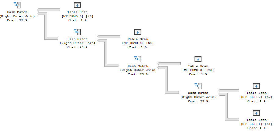
The first type of plan has hash joins which can all run concurrently. Memory for the hash tables cannot be reused between operators.

SQL Server Query Plan
bushy

For that query, the MF_DEMO_1 table is the probe side for all of the joins. SQL Server builds all of the hash joins and then rows flow from the probe side through the plan (as long as there aren’t tempdb spills). I will refer to this type of plan as a “concurrent join plan” which is a term that I just made up.

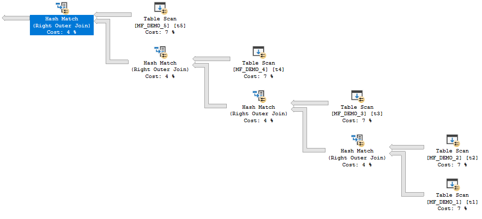
The second type of plan has hash joins which cannot all run concurrently. Pairs of hash tables are active at the same time, but memory grants can be reused between operators.

SQL Server Query Plans
not bushy

For that query, the MF_DEMO_1 table is the build side for all of the joins. Each hash table blocks the next one from starting. This means that at most two hash tables need to be kept in memory at the same time. Query memory cannot be reused for joins 1 and 2 but join 3 can reuse memory from join 1 and join 4 can reuse memory from join 2. I will refer to this type of plan as a “nonconcurrent join plan” which is another term that I just made up.

If the above wasn’t clear I recommend running through the demos with live query statistics enabled. It can be very useful to understand how rows flow through a plan. As far as I know, all queries of this type can be implemented with the nonconcurrent pattern but not all queries can be implemented with the concurrent pattern .

Create the Tables


The table definitions for our demos are pretty boring. I’m using a VARCHAR(100) as the join column to blow up memory grants and requirements a bit. All of the tables are heaps and have about 6.5 million rows in them. TARGET_TABLE is used as a dumping ground for the inserts and #ADD_BATCH_MODE is used to switch the hash joins to batch mode as desired. All testing was done on SQL Server 2016 SP1 CU7.

DROP TABLE IF EXISTS MF_DEMO_1;
CREATE TABLE MF_DEMO_1 (
       ID VARCHAR(100)
);

INSERT INTO MF_DEMO_1 WITH (TABLOCK)
SELECT 999999999999999 + ROW_NUMBER()
	OVER (ORDER BY (SELECT NULL))
FROM master..spt_values t1
CROSS JOIN master..spt_values t2;

CREATE STATISTICS S1 ON MF_DEMO_1 (ID) WITH FULLSCAN;

DROP TABLE IF EXISTS MF_DEMO_2;
CREATE TABLE MF_DEMO_2 (
       ID VARCHAR(100)
);

INSERT INTO MF_DEMO_2 WITH (TABLOCK)
SELECT 999999999999999 + ROW_NUMBER()
	OVER (ORDER BY (SELECT NULL))
FROM master..spt_values t1
CROSS JOIN master..spt_values t2;

CREATE STATISTICS S2 ON MF_DEMO_2 (ID) WITH FULLSCAN;

DROP TABLE IF EXISTS MF_DEMO_3;
CREATE TABLE MF_DEMO_3 (
       ID VARCHAR(100)
); 

INSERT INTO MF_DEMO_3 WITH (TABLOCK)
SELECT 999999999999999 + ROW_NUMBER()
	OVER (ORDER BY (SELECT NULL))
FROM master..spt_values t1
CROSS JOIN master..spt_values t2;

CREATE STATISTICS S3 ON MF_DEMO_3 (ID) WITH FULLSCAN;

DROP TABLE IF EXISTS MF_DEMO_4;
CREATE TABLE MF_DEMO_4 (
       ID VARCHAR(100)
); 

INSERT INTO MF_DEMO_4 WITH (TABLOCK)
SELECT 999999999999999 + ROW_NUMBER()
	OVER (ORDER BY (SELECT NULL))
FROM master..spt_values t1
CROSS JOIN master..spt_values t2;

CREATE STATISTICS S4 ON MF_DEMO_4 (ID) WITH FULLSCAN;

DROP TABLE IF EXISTS MF_DEMO_5;
CREATE TABLE MF_DEMO_5 (
	ID VARCHAR(100)
); 

INSERT INTO MF_DEMO_5 WITH (TABLOCK)
SELECT 999999999999999 + ROW_NUMBER()
	OVER (ORDER BY (SELECT NULL))
FROM master..spt_values t1
CROSS JOIN master..spt_values t2;

CREATE STATISTICS S5 ON MF_DEMO_5 (ID) WITH FULLSCAN;

CREATE TABLE #ADD_BATCH_MODE (I INT, INDEX CCI CLUSTERED COLUMNSTORE);

DROP TABLE IF EXISTS TARGET_TABLE;

CREATE TABLE TARGET_TABLE (ID VARCHAR(100));

Row Mode Memory Fractions For Concurrent Join Plans


The following query results in a concurrent join plan with row mode hash joins:

INSERT INTO TARGET_TABLE WITH (TABLOCK)
SELECT t1.ID
FROM MF_DEMO_3 t3
RIGHT OUTER JOIN MF_DEMO_2 t2
RIGHT OUTER JOIN MF_DEMO_1 t1
ON t1.ID = t2.ID
ON t1.ID = t3.ID
OPTION (FORCE ORDER, MAXDOP 1);

The desired memory grant is 2860640 KB. The memory fractions for both join operators have an input of 0.5 and an output of 0.5. This is exactly as expected. The hash tables can both start at the same time and cannot reuse memory, so each operator gets 50% of the query memory grant for the plan. Adding a third join to the plan increases the query memory grant to 4290960 KB.

INSERT INTO TARGET_TABLE WITH (TABLOCK)
SELECT t1.ID
FROM MF_DEMO_4 t4
RIGHT OUTER JOIN MF_DEMO_3 t3
RIGHT OUTER JOIN MF_DEMO_2 t2
RIGHT OUTER JOIN MF_DEMO_1 t1
ON t1.ID = t2.ID
ON t1.ID = t3.ID
ON t1.ID = t4.ID
OPTION (FORCE ORDER, MAXDOP 1);

Again, this seems very reasonable. SQL Server now tries to builds three hash tables in memory at the same time. The memory fractions for each operator have fallen to 0.3333333. Each operator gets a third of the query memory grant.

Row Mode Memory Fractions For Nonconcurrent Join Plans


The following query results in a nonconcurrent join plan with row mode hash joins:

INSERT INTO TARGET_TABLE WITH (TABLOCK)
SELECT t1.ID
FROM MF_DEMO_1 t1
INNER JOIN MF_DEMO_2 t2 ON t1.ID = t2.ID
INNER JOIN MF_DEMO_3 t3 ON t2.ID = t3.ID
INNER JOIN MF_DEMO_4 t4 ON t3.ID = t4.ID
OPTION (MAXDOP 1, FORCE ORDER);

The query plan was uploaded here. I recommend downloading the all of the plans referenced in this blost post if you’re interested in them so you can see all of the details.

Here are the memory fractions for the rightmost join (node 3):

Memory Fractions Input: 1, Memory Fractions Output: 0.476174

here are the memory fractions for the middle join (node 2):

Memory Fractions Input: 0.523826, Memory Fractions Output: 0.5

and here are the memory fractions for the leftmost join (node 1):

Memory Fractions Input: 0.5, Memory Fractions Output: 1

What do all of those numbers mean? The rightmost join builds its hash table first and starts with all query memory available to it. However, the output fraction is 0.476174. That means that the hash table can only use up to 47.6% of the query memory granted to the plan. The middle join is able to use up to 50% (the minimum of the input and output fractions for the node) of the memory granted to the plan. Note that 0.476174 + 0.523826 = 1.0. The last join to start executing is also able to use up to 50% of the granted memory. That join is the last operator that uses memory in the plan so the output fraction is 1.0. Memory grant reuse allows the plan to use up to 147.6% of the memory grant over the lifetime of the query execution. Without memory grant reuse each operator wouldn’t be able to use as much memory.

Removing one of the joins results in the desired query memory grant dropping from 3146704 KB to 3003672 KB. This is a significantly less drop than the other query. The smaller decrease is expected because the third join that we added can reuse the memory grant from the first. As more joins are added to a nonconcurrent plan the desired memory grant grows at a much slower rate than the memory grant for the concurrent join plan.

Batch Mode Memory Fractions For Concurrent Join Plans


The query plan for the next query is somewhat dependent on hardware. On my machine I had to let it run in parallel to get batch mode hash joins:

INSERT INTO TARGET_TABLE WITH (TABLOCK)
SELECT t1.ID
FROM MF_DEMO_5 t5
RIGHT OUTER JOIN MF_DEMO_4 t4
RIGHT OUTER JOIN MF_DEMO_3 t3
RIGHT OUTER JOIN MF_DEMO_2 t2
RIGHT OUTER JOIN MF_DEMO_1 t1
LEFT OUTER JOIN #ADD_BATCH_MODE ON 1 = 0
ON t1.ID = t2.ID
ON t1.ID = t3.ID
ON t1.ID = t4.ID
ON t1.ID = t5.ID
OPTION (FORCE ORDER, MAXDOP 4);

The estimated plan is here. It’s easy to tell if the query is using batch mode joins because the joins are run in parallel but there are no repartition stream operators.

SQL Server Query Plan
parallel and bushy

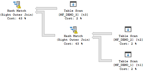
SQL Server is not able to reuse memory grants for this query. SQL Server tries to build all of the hash tables in memory before probe side is processed. However, the memory fractions are different from before: 0.25, 0.5, 0.75, and 1.0. These memory fractions do not make sense if interpreted in the same way as before. How can the final hash join in the plan have an input memory fraction of 1.0?

It’s unclear what the memory fractions are supposed to mean here, but there is one observable difference compared to the row mode plan. In the row mode equivalent plan SQL Server divides the memory evenly between operators. For our very simple test plan this means that all of the hash joins will spill to tempdb or none of them will spill. Reducing a MAX_GRANT_PERCENT hint from the right value by 1% results in two spills:

SQL Server Query Plan
spilly

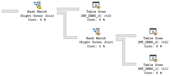
Both operators spilled because memory was divided evenly and there wasn’t enough memory to hold both hash tables in memory. However, with batch mode hash joins we can get plans like the following:

SQL Server Query Plan
spilly

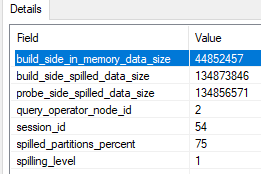
How is it possible that one join spills but the other doesn’t? It is only possible if memory isn’t divided evenly. It appears that memory is used as needed in some situations. Unfortunately, the actual plan for batch mode operators doesn’t give us a lot of spill information like it does for row mode. There’s a debug channel extended event query_execution_batch_hash_join_spilled that can give us some clues. 657920 KB of memory was granted for a two batch mode hash join query. For the operator that spilled, only 44852457 bytes were written to memory on the build side. That’s about 43800 KB, which is significantly less than half of available query memory.

SQL Server Extended Events
spills!

We can’t conclude that exactly 44852457 bytes of memory were granted to the operator. However, it should be somewhat close. In conclusion, for these types of queries it isn’t clear what the memory grant fractions are supposed to mean. SQL Server is able to exceed them in some cases. It’s possible to see 0 bytes of memory used for the build side in the extended event. I believe that this is the bad type of memory reuse as opposed to the good kind.

Batch Mode Memory Fractions For Nonconcurrent Join Plans


The following query results in a nonconcurrent batch mode hash join plan on my machine:

INSERT INTO TARGET_TABLE WITH (TABLOCK)
SELECT t1.ID
FROM MF_DEMO_1 t1
LEFT OUTER JOIN #ADD_BATCH_MODE On 1 = 0
WHERE EXISTS (
	SELECT 1
	FROM MF_DEMO_2 t2 WHERE t1.ID = t2.ID
) AND EXISTS (
	SELECT 1
	FROM MF_DEMO_3 t3 WHERE t1.ID = t3.ID
) AND EXISTS (
	SELECT 1
	FROM MF_DEMO_4 t4 WHERE t1.ID = t4.ID
) AND EXISTS (
	SELECT 1
	FROM MF_DEMO_5 t5 WHERE t1.ID = t5.ID
) OPTION (MAXDOP 4, FORCE ORDER);

As far as I know there’s nothing special about the semijoins. I used them to keep the estimated row size as consistent as possible. The behavior detailed below can be observed with normal joins as well.

Here is the estimated query plan. The same memory fraction pattern of 0.25, 0.50, 0.75, and 1.00 can be found in this query. Based on the query’s structure, memory grant reuse should be allowed between operators. Alarmingly, this query has the same desired memory grant as one with four concurrent joins. The desired memory grant changes significantly as tables are added or removed. This is a big change in behavior compared to row mode batch joins.

As far as I can tell, memory grant reuse can happen in plans like this with batch mode hash joins. Removing or adding joins results in very small adjustments in maximum memory used during query execution. Still, it seems as if the query optimizer is assuming that memory cannot be reused. With this query pattern, the first operator to run does not have access more memory implied by the memory fraction. In fact, it has access to less memory implied by the memory fraction.

Running the query without any memory grant hints results in no tempdb spills and a maximum memory use of 647168 KB. Restricting the memory grant to 2 GB results in a tempdb spill for the rightmost operator. This is unexpected. 500000 KB of memory should be more than enough memory to avoid a spill. As before, the only way I could find to investigate this further was to use the query_execution_batch_hash_join_spilled extended event and to force tempdb spills using the MAX_GRANT_PERCENT query hint.

A good amount of testing suggested that the available memory per operator is the input memory fraction for that operator divided by the sum of all output memory fractions. The rightmost operator only gets 0.25 / (0.25 + 0.5 + 0.75 + 1.0) = 10% of the memory granted to the query, the next operator gets 20%, the next operator gets 30%, and the final operator gets 40%. The situation gets worse as more joins are added to the query. Keep in mind that we aren’t doing anything tricky with cardinality estimates or data types which would result in skewed estimates. The query optimizer seems to recognize that each join will require the same amount of memory for each hash join, but it doesn’t make the same minimum amount available for each operator. That’s what is so puzzling.

The preceding paragraph seems to contradict the idea that memory grant reuse is possible for these plan shapes. Perhaps for these simple plans memory grant reuse is possible but it cannot go above 100% like we saw in the row mode plan. This could still be helpful in that the query could steal less memory from the buffer pool, but it’s certainly not as helpful in avoiding spills as the behavior we get with the row mode plan. Under the assumption the total memory grants seem a bit more reasonable, although it’s hard not to object as to how SQL Server is distributing the memory to each operator.

We can avoid the spill by giving SQL Server the memory that it required, but this is undesirable if multiple concurrent queries are running. I’ve often observed higher than expected memory grants for queries with batch mode hash joins. An assumption that query memory reuse will not be available for batch mode hash joins can explain part of what I’ve observed. If memory grants are left unchecked, applications may see decreased possible concurrency due to RESOURCE_SEMAPHORE waits. Lowering memory grants through any available method can result in unnecessary (based on total memory granted) tempdb spills. It’s easy to get stuck between a rock and a hard place.

Batch Mode Workarounds


There is some hope for nonconcurrent batch mode hash join plans. SQL Server 2017 introduces adaptive memory feedback for these operators. I imagine that functionality is a poor fit for ETL queries which may process dramatically different amounts of data each day, so I can’t view it as a complete solution. It certainly doesn’t help us on SQL Server 2016. Are there workarounds to prevent spills without requiring excessive memory grants? Yes, but they are very ugly and I can only imagine using them when truly needed during something like an ETL process.

Consider the following query:

INSERT INTO TARGET_TABLE WITH (TABLOCK)
SELECT t1.ID
FROM MF_DEMO_1 t1
LEFT OUTER JOIN MF_DEMO_2 t2 ON t2.ID = t1.ID
LEFT OUTER JOIN MF_DEMO_3 t3 ON t3.ID = t2.ID
LEFT OUTER JOIN MF_DEMO_4 t4 ON t4.ID = t3.ID
LEFT OUTER JOIN MF_DEMO_4 t5 ON t5.ID = t4.ID
LEFT OUTER JOIN #ADD_BATCH_MODE ON 1 = 0
OPTION (FORCE ORDER, MAXDOP 4, MAX_GRANT_PERCENT = 60);

On my machine, the memory hint results in a memory grant of 2193072 KB. The rightmost join spills even when only a maximum of 1232896 KB of memory is used during query execution:

SQL Server Query Plan
more spills!

One way to avoid the spill is to shift the memory fractions in our favor. Ideally SQL Server would think that the rightmost join would need much more memory for its hash table than the other joins. If we can add an always NULL column with a large data type that is only needed for the first hash table, that might do the trick. The query syntax below isn’t guaranteed to get the plan that we want but it seems to work in this case:

ALTER TABLE MF_DEMO_1 ADD DUMMY_COLUMN_V4000 VARCHAR(4000) NULL;
ALTER TABLE MF_DEMO_2 ADD DUMMY_COLUMN_V10 VARCHAR(10) NULL;

INSERT INTO TARGET_TABLE WITH (TABLOCK)
SELECT t1.ID
FROM MF_DEMO_1 t1
LEFT OUTER JOIN MF_DEMO_2 t2 ON t2.ID = t1.ID
LEFT OUTER JOIN MF_DEMO_3 t3 ON t3.ID = t2.ID
LEFT OUTER JOIN MF_DEMO_4 t4 ON t4.ID = t3.ID
LEFT OUTER JOIN MF_DEMO_4 t5 ON t5.ID = t4.ID
LEFT OUTER JOIN #ADD_BATCH_MODE ON 1 = 0
WHERE (t1.DUMMY_COLUMN_V4000 IS NULL OR t2.DUMMY_COLUMN_V10 IS NULL)
OPTION (FORCE ORDER, MAXDOP 4, MAX_GRANT_PERCENT = 32);

An actual plan was uploaded here. The query no longer spills even though the memory grant was cut to 1225960 KB. The memory fractions are now 0.82053, 0.878593, 0.936655, and 1. The change was caused by the increase in estimated row size for the rightmost join: 2029 bytes. That row size is reduced to 45 bytes after the filter is applied, which won’t filter out any rows because both columns are always NULL. The FORCE ORDER hint is essential to get this plan shape. It’s very unnatural otherwise.

If the same rules are followed as before, the rightmost join should get 22.5% of the available query memory grant now. This is enough to avoid the spill to tempdb.

Final Thoughts


I understand that the formulas for memory fractions need to account for an arbitrary combination of row mode and batch mode operators in a query plan. However, it is disappointing that the available information for memory fractions for batch mode operators is so confusing, some queries with batch mode hash joins ask for way more memory than they need, and some queries needlessly spill to tempdb without using close to their full memory grant. Batch mode adaptive memory grant feedback can offer some relief in SQL Server 2017, but why not expect good plans the first time as long as we’re giving the query optimizer good information?

Thanks for reading!

Going Further


If this is the kind of SQL Server stuff you love learning about, you’ll love my training. Blog readers get 25% off the Everything Bundle — over 100 hours of performance tuning content. Need hands-on help? I offer consulting engagements from targeted investigations to ongoing retainers. Want a quick sanity check before committing to a full engagement? Schedule a call — no commitment required.

SQL Server Join Containment for the Common Man

Lots of smart people have written about join containment, but none of the explanations really made sense to me. I felt like a student memorizing definitions for a test. Sure, I could tell you the definitions of base and simple containment, but what practical difference does it make when it comes to cardinality estimation? The concept finally clicked when working on an Oracle query of all things, and as a result I wrote this blog post. All testing was done on SQL Server 2017 with a CE version of 140.

A Note on Join Cardinality


Join cardinality calculations are incredibly complex in SQL Server. You can get a small taste of that complexity here. I’ve chosen the example data in this blog post to avoid most of the complexity. The formulas and concepts described in this post can’t be used to model join cardinality generally, but I hope that they serve as a good illustration of containment.

Demo Tables


All of the demo tables have identical structures with similar data. The first column, UNIQUE_ID, stores unique integers in the range specified in the table name. For example, TA_1_TO_1000000 is a table that stores integers from 1 to 1000000. The second column, MOD_FILTER, stores integers from 1 to 100 cycling through all rows. The purpose of this column is to make filtering cardinality estimates simple to calculate and predict. For example, MOD_FILTER BETWEEN 1 AND 50 will return 50% of the rows from the table. Full statistics are gathered on all columns, and there are four tables in all.

DROP TABLE IF EXISTS dbo.TA_1_TO_1000000;

CREATE TABLE dbo.TA_1_TO_1000000 (
	UNIQUE_ID BIGINT NOT NULL,
	MOD_FILTER BIGINT NOT NULL
);

INSERT INTO dbo.TA_1_TO_1000000
	WITH (TABLOCK)
SELECT t.RN
, 1 + t.RN % 100
FROM
(
	SELECT TOP (1000000) ROW_NUMBER()
		OVER (ORDER BY (SELECT NULL)) RN
	FROM master..spt_values t1
	CROSS JOIN master..spt_values t2
) t
OPTION (MAXDOP 1);

CREATE STATISTICS S1 ON dbo.TA_1_TO_1000000 (UNIQUE_ID)
	WITH FULLSCAN;
CREATE STATISTICS S2 ON dbo.TA_1_TO_1000000 (MOD_FILTER)
	WITH FULLSCAN;

DROP TABLE IF EXISTS dbo.TB_1_TO_1000000;

CREATE TABLE dbo.TB_1_TO_1000000 (
	UNIQUE_ID BIGINT NOT NULL,
	MOD_FILTER BIGINT NOT NULL
);

INSERT INTO dbo.TB_1_TO_1000000
	WITH (TABLOCK)
SELECT t.RN
, 1 + t.RN % 100
FROM
(
	SELECT TOP (1000000) ROW_NUMBER()
		OVER (ORDER BY (SELECT NULL)) RN
	FROM master..spt_values t1
	CROSS JOIN master..spt_values t2
) t
OPTION (MAXDOP 1);

CREATE STATISTICS S1 ON dbo.TB_1_TO_1000000 (UNIQUE_ID)
	WITH FULLSCAN;
CREATE STATISTICS S2 ON dbo.TB_1_TO_1000000 (MOD_FILTER)
	WITH FULLSCAN;

DROP TABLE IF EXISTS dbo.TC_1_TO_100000;

CREATE TABLE dbo.TC_1_TO_100000 (
	UNIQUE_ID BIGINT NOT NULL,
	MOD_FILTER BIGINT NOT NULL
);

INSERT INTO dbo.TC_1_TO_100000
	WITH (TABLOCK)
SELECT t.RN
, 1 + t.RN % 100
FROM
(
	SELECT TOP (100000) ROW_NUMBER()
		OVER (ORDER BY (SELECT NULL)) RN
	FROM master..spt_values t1
	CROSS JOIN master..spt_values t2
) t
OPTION (MAXDOP 1);

CREATE STATISTICS S1 ON dbo.TC_1_TO_100000 (UNIQUE_ID)
	WITH FULLSCAN;
CREATE STATISTICS S2 ON dbo.TC_1_TO_100000 (MOD_FILTER)
	WITH FULLSCAN;

DROP TABLE IF EXISTS dbo.TD_500001_TO_1500000;

CREATE TABLE dbo.TD_500001_TO_1500000 (
	UNIQUE_ID BIGINT NOT NULL,
	MOD_FILTER BIGINT NOT NULL
);

INSERT INTO dbo.TD_500001_TO_1500000
	WITH (TABLOCK)
SELECT t.RN
, 1 + t.RN % 100
FROM
(
	SELECT TOP (1000000) 500000 + ROW_NUMBER()
		OVER (ORDER BY (SELECT NULL)) RN
	FROM master..spt_values t1
	CROSS JOIN master..spt_values t2
) t
OPTION (MAXDOP 1);

CREATE STATISTICS S1 ON dbo.TD_500001_TO_1500000 (UNIQUE_ID)
	WITH FULLSCAN;
CREATE STATISTICS S2 ON dbo.TD_500001_TO_1500000 (MOD_FILTER)
	WITH FULLSCAN;

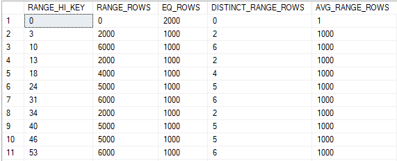
The statistics objects are perfect in that they fully describe the data. Here’s the statistics output for the UNIQUE_ID column:
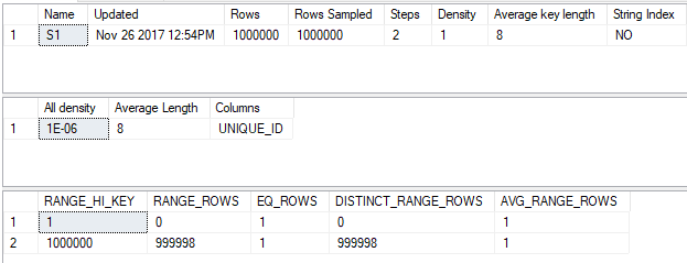
a21_T2_perfect_stats_1

And here’s the output for the MOD_FILTER column:
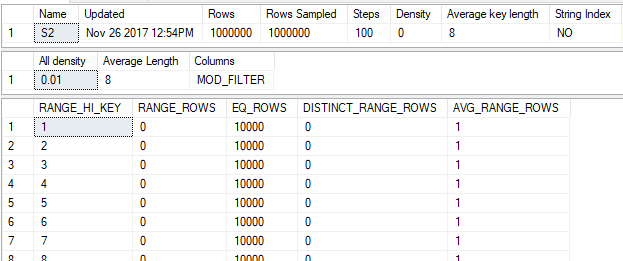
a21_T2_perfect_stats_2

This only happened because the table was populated with very simple data that fits well within the framework for generating histograms in SQL Server. Gathering statistics, even with FULLSCAN, will often not perfectly represent the data in the column.

A Simple Model of Join Cardinality Estimation


Consider the following simple query:

SELECT *
FROM TB_1_TO_1000000 b
INNER JOIN dbo.TD_500001_TO_1500000 d
	ON b.UNIQUE_ID = d.UNIQUE_ID;

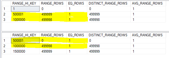
We know that exactly 500000 rows will be returned, but how might SQL Server estimate the number of rows to be returned? Let’s look at the histograms and try to align their steps:
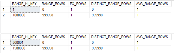
a21_ex1_not_aligned

That doesn’t exactly work, but we can split up the histogram steps so they align. The assumption of uniformity within the step isn’t even needed here because we know that there aren’t missing any integer values. The histograms below are equivalent to the original ones:
a21_ex1_aligned

Now the RANGE_HI_KEY values align. For the step with a high value of 500001 we can expect only one row to match between tables. For the step with a high value of 1000000 we can expect 499998 + 1 rows to match. This brings the total row estimate to 500000, which happens to match what I get in SQL Server 2017 with the new CE. Remember, what we’re doing here isn’t how the query optimizer does the calculation. This is just a simple model that will be useful later.

Now consider the two queries below:

SELECT *
FROM TA_1_TO_1000000 a
INNER JOIN dbo.TB_1_TO_1000000 b
	ON a.UNIQUE_ID = b.UNIQUE_ID
WHERE a.MOD_FILTER BETWEEN 1 AND 50
AND b.MOD_FILTER BETWEEN 1 AND 50;

SELECT *
FROM TA_1_TO_1000000 a
INNER JOIN dbo.TB_1_TO_1000000 b
	ON a.UNIQUE_ID = b.UNIQUE_ID
WHERE a.MOD_FILTER BETWEEN 1 AND 50
AND b.MOD_FILTER BETWEEN 51 AND 100;

We know that the first query will return 500k rows and the second query will return 0 rows. However, can SQL Server know that? Each statistics object only contains information about its own column. There’s no correlation between the UNIQUE_ID and MOD_FILTER columns, so there isn’t a way for SQL Server to know that the queries will return different estimates. The query optimizer can create an estimate based on the filters on the WHERE clause and on the histograms of the join columns, but there’s no foolproof way to do that calculation. The presence of the filters introduces uncertainty into the estimate, even with statistics that perfectly describe the data for each column. The containment assumption is all about the modeling assumption that SQL Server has to make to resolve that uncertainty.

Base Containment


Base containment is the assumption that the filter predicates are independent from the join selectivity. The estimate for the join should be obtained by multiplying together the selectivity from both filters and the join. The query optimizer uses base containment starting with CE model version 120, also known as the new CE introduced in SQL Server 2014. It can be used with the legacy CE if trace flag 2301 is turned on. The best reference for trace flag 2301 is a blog post from 2006 which is no longer published.

Let’s go back to this example query:

SELECT *
FROM TA_1_TO_1000000 a
INNER JOIN dbo.TB_1_TO_1000000 b
	ON a.UNIQUE_ID = b.UNIQUE_ID
WHERE a.MOD_FILTER BETWEEN 1 AND 50
AND b.MOD_FILTER BETWEEN 1 AND 50;

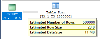
The selectivity for the filter on MOD_FILTER is 0.5 for both tables. This is because there are 100 unique values for MOD_FILTER between 1 and 100 and each value matches 1% of the table. We can see this by getting an estimated query plan on just TA_1_TO_1000000:
a21_ex2_filter_selectivity

The table has 1 million rows, so the estimate is 500000 = 0.5 * 1000000.

That leaves the join selectivity. We put the same data into both tables:
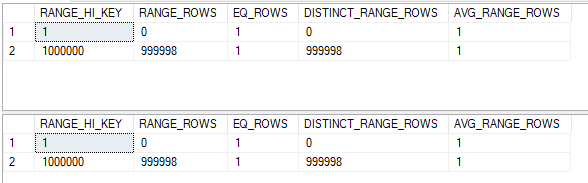
a21_ex2_same_histograms

We don’t need highlighters to see that the join selectivity is 1.0.

Putting it all together, the cardinality estimate under base containment for this query should be 1000000 * 1.0 * 0.5 * 0.5 = 250000. This is indeed the estimate:
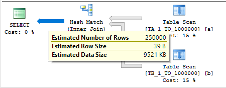
a21_ex2_base_estimate

Of course, this doesn’t match the actual number of rows which is 500000. But it’s easy to change the filter predicates so that the estimated number of rows and the actual number of rows match.

Simple Containment


Simple containment is the assumption that the filter predicates are not independent. The estimate for the join should be obtained by applying the filter selectivities to the join histograms and joining based on the adjusted histograms. The query optimizer uses simple containment within the legacy CE. Simple containment can be used in the new CE via trace flag or USE HINT.

Let’s go back to the same example query:

SELECT *
FROM TA_1_TO_1000000 a
INNER JOIN dbo.TB_1_TO_1000000 b
	ON a.UNIQUE_ID = b.UNIQUE_ID
WHERE a.MOD_FILTER BETWEEN 1 AND 50
AND b.MOD_FILTER BETWEEN 1 AND 50
OPTION (
USE HINT ('ASSUME_JOIN_PREDICATE_DEPENDS_ON_FILTERS')
);

We know that the filter selectivity for both tables is 0.5. How can that be used to adjust the histograms? The simplest method would be to just multiply RANGE_ROWS, EQ_ROWS, and DISTINCT_RANGE_ROWS by the filter selectivity. After doing so we’re left with two still identical histograms:
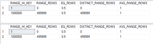
a21_ex2_simple_histograms

It might seem odd to work with fractions of a row, but as long as everything is rounded at the end why should it matter? With two identical, aligned histograms it seems reasonable to expect a cardinality estimate of 0.5 + 499999 + 0.5 = 500000. This is exactly what we get in SQL Server:
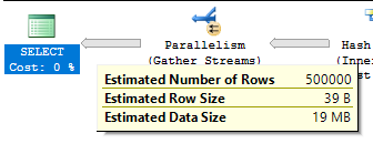
a21_ex2_simple_estimate

The actual row estimate matches the estimated row estimate because the filters are perfectly correlated. Every row left after filtering still has a matching row in the other table.

Just One Filter


What happens if we filter on just a single table? For example:

SELECT *
FROM dbo.TA_1_TO_1000000 a
INNER JOIN dbo.TB_1_TO_1000000 b
	ON a.UNIQUE_ID = b.UNIQUE_ID
WHERE a.MOD_FILTER BETWEEN 1 AND 30;

SELECT *
FROM dbo.TA_1_TO_1000000 a
INNER JOIN dbo.TB_1_TO_1000000 b
	ON a.UNIQUE_ID = b.UNIQUE_ID
WHERE a.MOD_FILTER BETWEEN 1 AND 30
OPTION (
USE HINT ('ASSUME_JOIN_PREDICATE_DEPENDS_ON_FILTERS')
);

For base containment, we know that the filter selectivity is 0.3 and the join selectivity is 1.0. We can expect a cardinality estimate of 1000000 * 1.0 * 0.3 = 300000 rows.

For simple containment we need to multiply the histogram for TA_1_TO_1000000 by 0.3. Here’s what the two histograms look like after factoring in filter selectivity:
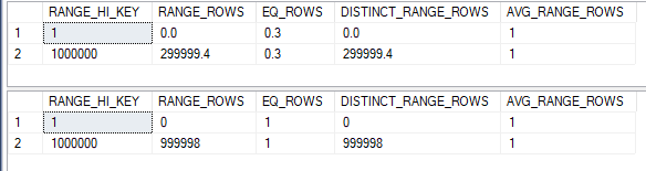
a21_ex3_simple_histograms

What should the estimate be? One approach would be to assume that everything matches between the aligned steps. So we end up with 0.3 rows from the step with a RANGE_HI_KEY of 1 and 299999.4 + 0.3 rows from the step with a RANGE_HI_KEY of 1000000. The combined estimate is 300000 rows, which matches the base containment estimate. Why shouldn’t they match? Without filters on both tables there’s no concept of correlation. If it helps you can imagine a filter of 1 = 1 on TB_1_TO_1000000. For base containment multiplying by 1.0 won’t change the estimate and for simple containment multiplying by 1 won’t change the histogram. That just leaves a single filter selectivity of 0.3 for TA_1_TO_1000000 and both estimates should be the same.

For both queries the estimated number of rows in SQL Server is 300000. Our calculations match the SQL Server query optimizer exactly for this query.

Filtering on the Join Column


What happens if we filter on the join columns of both tables? For example:

SELECT *
FROM dbo.TA_1_TO_1000000 a
INNER JOIN dbo.TB_1_TO_1000000 b
	ON a.UNIQUE_ID = b.UNIQUE_ID
WHERE a.UNIQUE_ID BETWEEN 1 AND 200000
AND b.UNIQUE_ID BETWEEN 1 AND 200000;

SELECT *
FROM dbo.TA_1_TO_1000000 a
INNER JOIN dbo.TB_1_TO_1000000 b
	ON a.UNIQUE_ID = b.UNIQUE_ID
WHERE a.UNIQUE_ID BETWEEN 1 AND 200000
AND b.UNIQUE_ID BETWEEN 1 AND 200000
OPTION (
USE HINT ('ASSUME_JOIN_PREDICATE_DEPENDS_ON_FILTERS')
);

Think back to why we need containment in the first place. When there are filters on columns that aren’t the join columns then we need to make an assumption as to how the selectivities all interact with each other. With a filter on the join column we can just adjust the histogram of the join column directly. There isn’t any uncertainty. Here’s what the histograms could look like:
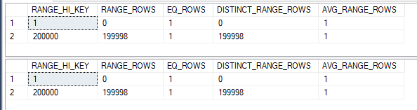
a21_ex4_histograms

In which case, it seems obvious that the final estimate should be 200000 rows. Simple containment does not result in a different estimate here.

Removing Rows


So far the examples have been very simple. We’ve joined tables that contain the exact same data. What if one table has fewer rows than the other table? Consider the following pair of queries:

SELECT *
FROM dbo.TC_1_TO_100000 c
INNER JOIN dbo.TB_1_TO_1000000 b
	ON c.UNIQUE_ID = b.UNIQUE_ID
WHERE c.MOD_FILTER BETWEEN 1 AND 50
AND b.MOD_FILTER BETWEEN 1 AND 50;

SELECT *
FROM dbo.TC_1_TO_100000 c
INNER JOIN dbo.TB_1_TO_1000000 b
	ON c.UNIQUE_ID = b.UNIQUE_ID
WHERE c.MOD_FILTER BETWEEN 1 AND 50
AND b.MOD_FILTER BETWEEN 1 AND 50
OPTION (
USE HINT ('ASSUME_JOIN_PREDICATE_DEPENDS_ON_FILTERS')
);

It’s important to call out here that TC_1_TO_100000 has just 100000 rows instead of one million. For base containment, we know that the selectivity will be 0.5 for both tables. What about join selectivity? The histogram steps of course aren’t aligned:
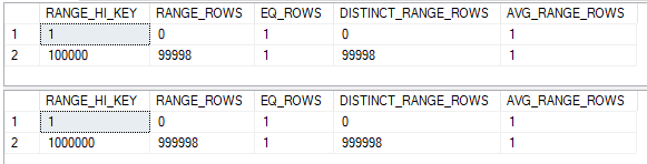
a21_ex5_initial_histograms

The data is densely packed, so we can use the same trick as before to split the histogram for the larger table:
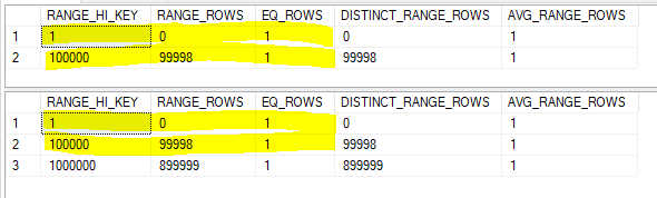
a21_ex5_base_aligned_histograms

Every row in histogram for the smaller table has a match in the histogram of the larger table. From the point of view of the smaller table the join selectivity is 1.0. Multiplying together all three selectivities gives a final row estimate of 100000 * 1.0 * 0.5 * 0.5 = 25000. This matches the row estimate within SQL Server exactly.

For simple containment we need to apply the filter selectivities of 0.5 to both tables. We also need to align the histograms by splitting the larger histogram. Both will be done in one step:
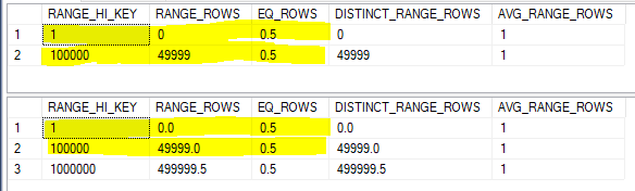
a21_ex5_simple_histograms

Every row in the smaller histogram once again matches. Our final estimate is 0.5 + 49999 + 0.5 = 50000 which exactly matches the SQL Server query optimizer.

Unmatched Rows


What happens if the tables have the same number of rows but they clearly don’t contain the same data? Consider the following pair of queries:

SELECT *
FROM dbo.TD_500001_TO_1500000 d
INNER JOIN dbo.TB_1_TO_1000000 b
	ON d.UNIQUE_ID = b.UNIQUE_ID
WHERE d.MOD_FILTER BETWEEN 1 AND 50
AND b.MOD_FILTER BETWEEN 1 AND 10;

SELECT *
FROM dbo.TD_500001_TO_1500000 d
INNER JOIN dbo.TB_1_TO_1000000 b
	ON d.UNIQUE_ID = b.UNIQUE_ID
WHERE d.MOD_FILTER BETWEEN 1 AND 50
AND b.MOD_FILTER BETWEEN 1 AND 10
OPTION (
USE HINT ('ASSUME_JOIN_PREDICATE_DEPENDS_ON_FILTERS')
);

The filter predicate for TB_1_TO_1000000 is 0.1 and the filter predicate for TD_500001_TO_1500000 is 0.5. Here are our starting histograms:
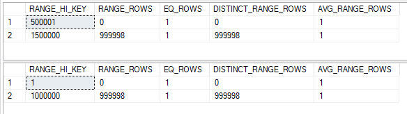
a21_ex6_base_initial_histograms

The little man who lives inside the cardinality estimator needs to slice them up so they align. His work is complete:
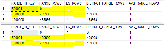
a21_ex6_base_sliced_histograms

The top histogram has 500000 unmatched rows in the step with a RANGE_HI_KEY of 1500000, so the join selectivity is 500000 / 1000000 = 0.5. Putting all three selectivities together, the cardinality estimate with base containment should be 1000000 * 0.5 * 0.1 * 0.5 = 25000. This exactly matches SQL Server.

You know the drill for simple containment. We need to multiply each sliced histogram by its filter selectivity:
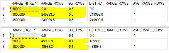
a21_ex6_simple_sliced_histograms

That’s pretty messy. I’m going to assume that every row has a match between the two shared steps, so the estimate should be 0.1 + 49999.8 + 0.1 = 50000. The number of estimated rows reported by SQL Server is 50000.4 :
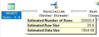
a21_ex6_simple_estimate

What happened? Did the little man only measure once before cutting? This is one of those examples where there’s other complicated stuff going on under the hood, so the predicted row estimate doesn’t match up exactly. Interestingly, the estimate with the legacy cardinality estimator is exactly 50000.

An Approximate Formula


  • Define T1_CARDINALITY as the number of rows in the first joined table.
  • Define T1_FILTER_SELECTIVITY as the filter selectivity of the filter predicates of the first table. This number ranges from 0.0 to 1.0, with 1.0 for filters that remove no rows.
  • Define T2_CARDINALITY as the number of rows in the second joined table.
  • Define T2_FILTER_SELECTIVITY as the filter selectivity of the filter predicates of the second table. This number ranges from 0.0 to 1.0, with 1.0 for filters that remove no rows.
  • Define JOIN_SELECTIVITY as the selectivity of the two histograms of the joined columns from the point of view of the smaller table. This number ranges from 0.0 to 1.0, with 1.0 meaning that all rows in the smaller table have a match in the larger table.

Based on the tests above, we can model the cardinality estimates for base and simple containment as follows:

Base containment = JOIN_SELECTIVITY * LEAST(T1_CARDINALITY, T2_CARDINALITY) * T1_FILTER_SELECTIVITY * T2_FILTER_SELECTIVITY
Simple containment = JOIN_SELECTIVITY * LEAST(T1_FILTER_SELECTIVITY * T1_CARDINALITY, T2_FILTER_SELECTIVITY * T2_CARDINALITY)

Remember that this isn’t how SQL Server actually does it. However, I think that it shows the difference between base containment and simple containment quite well. For simple containment the filters are applied to the histograms and for base containment all of the selectivities are independent.

A Mathematical Proof?


So far simple containment has always had a higher cardinality estimate than base containment. Looking at the formulas it certainly feels like simple should have a higher estimate. Can we prove that the estimate will always be higher using the above formulas? It’s been quite a few years so I apologize for the proof below, but I believe that it gets the job done.

Definitions:

JS = JOIN_SELECTIVITY
C1 = T1_CARDINALITY
F1 = T1_FILTER_SELECTIVITY
C2 = T2_CARDINALITY
F2 = T2_FILTER_SELECTIVITY

Attempt a proof by contradiction, so assume the opposite of what we want to prove:

JS * LEAST(C1, C2) * F1 * F2 > JS * LEAST(F1 * C1, F2 * C2)

We know that JS > 0, F1 > 0, and F2 > 0, so:

LEAST(C1, C2) > LEAST(C1 / F2, C2 / F1)

The left hand expression can only evalute to C1 or C2. Let’s assume that it evaluates to C1, so C1 <= C2. We know that F1 <= 1, so C2 <= C2 / F1. C1 / F2 > C1, so the only hope of the inequality above being true is if C1 > C2 / F1. Putting it all together:

C1 <= C2 <= C2 / F1 < C1

That is clearly impossible. Very similar logic holds if the left hand expression evaluates to C2 (just flip 1 with c in the above), so we know that the equation that we started out with is not true. Therefore:

JS * LEAST(C1, C2) * F1 * F2 <= JS * LEAST(F1 * C1, F2 * C2)

In other words:

BASE CONTAINMENT <= SIMPLE CONTAINMENT

Here’s my public domain celebration picture:

a21_anniversary-157248_960_720

The details of this stuff within SQL Server are very complicated, so this doesn’t mean that there doesn’t exist a query that has a larger cardinality estimate with base containment. However, it seems to be a safe assumption that in general simple containment will result in a larger or equal estimate compared to base containment.

Why Does Any of This Matter?


I almost created a kind of real life example here, but I ran out of time so you’re eating Zs for dinner again as usual. Let’s introduce a table to cause some trouble:

DROP TABLE IF EXISTS dbo.ROWGOAL_TROUBLES;

CREATE TABLE dbo.ROWGOAL_TROUBLES (
	UNIQUE_EVEN_ID BIGINT NOT NULL,
	PAGE_FILLER VARCHAR(1000) NOT NULL
);

INSERT INTO dbo.ROWGOAL_TROUBLES
	WITH (TABLOCK)
SELECT 2 * t.RN
, REPLICATE('Z', 1000)
FROM
(
	SELECT TOP (50000) ROW_NUMBER()
		OVER (ORDER BY (SELECT NULL)) / 100 RN
	FROM master..spt_values t1
	CROSS JOIN master..spt_values t2
) t
OPTION (MAXDOP 1);

Consider the following business critical query that I run all the time:

SELECT *
FROM dbo.TA_1_TO_1000000 t1
INNER JOIN dbo.TB_1_TO_1000000 t2
	ON t1.UNIQUE_ID = t2.UNIQUE_ID
WHERE t1.MOD_FILTER = 1
AND t2.MOD_FILTER = 1
AND NOT EXISTS (
	SELECT 1
	FROM dbo.ROWGOAL_TROUBLES rt
	WHERE rt.UNIQUE_EVEN_ID = t1.UNIQUE_ID
)
OPTION (MAXDOP 1);

The plan doesn’t look so hot:
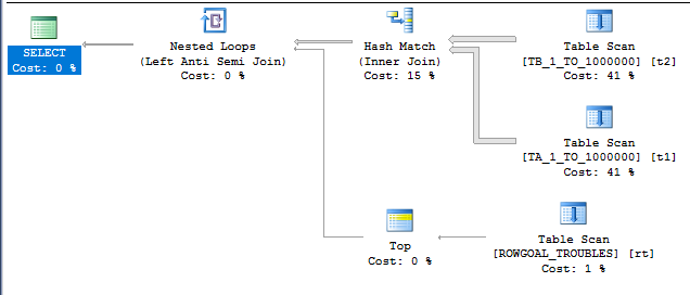
a21_bad_row_goal

There are unmatched rows in the ROWGOAL_TROUBLES table, so we know that the scan on the inner side of the nested loop is going to read a lot of rows. The query took about 60 seconds to finish on my machine and read 499775000 rows from the ROWGOAL_TROUBLES table. Why did this plan seem attractive to SQL Server? The query optimizer thought that only 100 rows would be returned after the join of TA_1_TO_1000000 to TB_1_TO_1000000. The filters are perfectly correlated so 10000 rows will be returned in reality. With perfectly correlated filters we can expect a better estimate if we use simple containment:

SELECT *
FROM dbo.TA_1_TO_1000000 t1
INNER JOIN dbo.TB_1_TO_1000000 t2
	ON t1.UNIQUE_ID = t2.UNIQUE_ID
WHERE t1.MOD_FILTER = 1
AND t2.MOD_FILTER = 1
AND NOT EXISTS (
	SELECT 1
	FROM dbo.ROWGOAL_TROUBLES rt
	WHERE rt.UNIQUE_EVEN_ID = t1.UNIQUE_ID
)
OPTION (
MAXDOP 1,
USE HINT ('ASSUME_JOIN_PREDICATE_DEPENDS_ON_FILTERS')
);

With a better estimate of 10000 rows comes a better query plan:
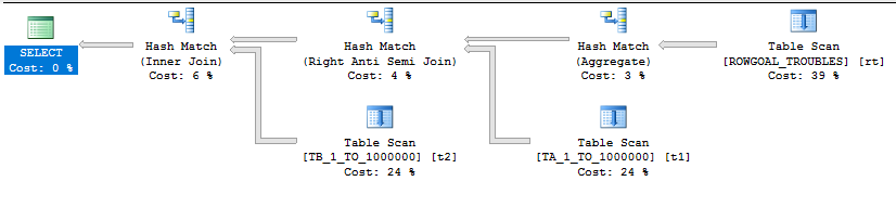
a21_no_row_goal

The query finishes in under a second on my machine.

Final Thoughts


Hopefully this blog post gives you a better understanding of the difference between base and simple containment. Read some of the other explanations out there if this wasn’t helpful. Containment is a tricky subject and you never know what it’ll take for it to make sense to you.

Thanks for reading!

Going Further


If this is the kind of SQL Server stuff you love learning about, you’ll love my training. Blog readers get 25% off the Everything Bundle — over 100 hours of performance tuning content. Need hands-on help? I offer consulting engagements from targeted investigations to ongoing retainers. Want a quick sanity check before committing to a full engagement? Schedule a call — no commitment required.
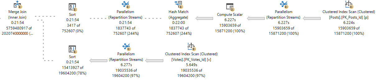

A Row Goal Request For SQL Server

If you don’t know about row goals I strongly recommend reading up on them here. Queries with plans similar to the following may sometimes take longer than expected to finish:

a16_suspicious_query

This can happen even in SQL Server 2017 with very representative statistics and perfect cardinality estimates. This post digs into why these performance degradations can happen and proposes a way to prevent them.

The Test Data


For test data I threw about a million rows into a heap. There are exactly 1000 unique values for the ID column. The table is about 1 GB in size.

DROP TABLE IF EXISTS dbo.BIG_HEAP;

CREATE TABLE dbo.BIG_HEAP (
	ID BIGINT NOT NULL,
	PAGE_FILLER VARCHAR(900) NOT NULL
);

-- table is about 1 GB in size
INSERT INTO dbo.BIG_HEAP WITH (TABLOCK)
SELECT
  RN
, REPLICATE ('Z', 900)
FROM
(
	SELECT TOP (1000000)
		ROW_NUMBER()
		OVER (ORDER BY (SELECT NULL)) % 1000 RN
	FROM master..spt_values t1
	CROSS JOIN master..spt_values t2

	UNION ALL

	SELECT TOP (1000) 0 RN
	FROM master..spt_values t1
	CROSS JOIN master..spt_values t2
) t
OPTION (MAXDOP 1);

CREATE STATISTICS S ON dbo.BIG_HEAP (ID)
WITH FULLSCAN, NORECOMPUTE;

The histogram isn’t as compact as it theoretically could be, but I would say that it represents the data very well:

a16_rowstore_histogram

Through the histogram it’s easy to see that there are 1000 distinct values for the ID column. There are 2000 rows with an ID of 0 and 1000 rows for IDs between 1 and 999.

The data is evenly distributed on disk. This behavior isn’t guaranteed because we’re inserting into a heap, but what counts is that it remains true during the testing period. We can get the first row with any ID in the table by reading 1000 rows or fewer from the heap. Below are a few examples:

-- rows read from table = 1
SELECT TOP (1) ID
FROM dbo.BIG_HEAP
WHERE ID = 1;

-- rows read from table = 500
SELECT TOP (1) ID
FROM dbo.BIG_HEAP
WHERE ID = 500;

-- rows read from table = 999
SELECT TOP (1) ID
FROM dbo.BIG_HEAP
WHERE ID = 999;

-- rows read from table = 1000
SELECT TOP (1) ID
FROM dbo.BIG_HEAP
WHERE ID = 0;

Approximate Formula for Scan Costing with a Row Goal


After some investigation I was able to come up with an approximate formula for the cost of a scan with a row goal applied to it. The formula has rounding and other issues but it illustrates the general behavior quite well. Here it is:

scan cost in optimizer units = 0.0031895 + LEAST(1, ROW_GOAL / CARDINALITY_ESTIMATE) * (FULL_SCAN_COST – 0.0031895)

I assume that the 0.0031895 constant is there to represent the minimum amount of work required to read a single row from a table. The ROW_GOAL parameter will just be the number of rows limited by TOP in our example queries. The CARDINALITY_ESTIMATE parameter is the number of rows estimated to be returned by SQL Server if there was no row goal. The FULL_SCAN_COST parameter is the cost in optimizer units of a single scan that reads all of the rows from the table. For BIG_HEAP this has a value of 93.7888.

SQL Server assumes that rows are evenly distributed in the table when reducing the cost of the scan. It’s certainly possible to take issue with that assumption, but this blog post does not go in that direction. In fact, I loaded the data into BIG_HEAP in such a way so that assumption would be largely true. The basic idea behind the formula is that if there are two matching rows in a table and a query needs to get just one of them, then on average the query optimizer thinks that half of the rows will need to be read from the table.

Let’s start with a few simple examples. If a row goal exceeds the total number of rows in a table then we shouldn’t expect it to change the cost of a scan. For this query:

SELECT TOP (7654321) ID
FROM dbo.BIG_HEAP;

The formula simplifies to 0.0031895 + (1) * (93.7888 - 0.0031895) = 93.7888 units which is exactly the cost of the scan.

Consider a query that selects the first row without any filtering:

SELECT TOP (1) ID
FROM dbo.BIG_HEAP;

The ROW_GOAL is 1 and the CARDINALITY_ESTIMATE is the number of rows in the table, 1001000. The formula gives a cost of 0.0031895 + (1 / 1001000) * (93.7888 - 0.0031895) = 0.00328319191 units which is fairly close to the actual cost of 0.0032831 units.

The formula also works for the classic SELECT TOP (0) query. The query below does not contain a scan of the heap so it could be said that the cost of the scan is 0 units.

SELECT TOP (0) ID
FROM dbo.BIG_HEAP;

For a less trivial example consider the following query:

SELECT TOP (3) ID
FROM dbo.BIG_HEAP
WHERE ID = 1;

The ROW_GOAL is 3 and the CARDINALITY_ESTIMATE is 1000. The formula gives a cost of 0.0031895 + (3 / 1000) * (93.7888 - 0.0031895) = 0.2845463315 units. The scan cost reported by SQL Server is 0.284546 units.

Consider the following query:

SELECT TOP (1) ID
FROM dbo.BIG_HEAP
WHERE ID = 0;

The ROW_GOAL is 1 and the CARDINALITY_ESTIMATE is 2000. The formula gives a cost of 0.0031895 + (1 / 2000) * (93.7888 - 0.0031895) = 0.05008230525 units. The scan cost reported by SQL Server is 0.0500822 units.

An estimate based on density gives what you might expect. Consider the following query:

DECLARE @var BIGINT = 1;
SELECT TOP (1) ID
FROM dbo.BIG_HEAP
WHERE ID = @var
OPTION (MAXDOP 1);

Here the cardinality estimate will be 1001 rows. The formula gives a cost of 0.0031895 + (1 / 1001) * (93.7888 - 0.0031895) = 0.09688141858 units. The scan cost reported by SQL Server is 0.0968814 units.

Approximate Formula for Join Scan Costing with a Row Goal


The truly interesting part is how the scan cost changes due to a row goal when it’s on the inner side of a nested loop join. To model the cost we need to make a few changes to the above formula. First we need a way to approximate the cost of each successive scan. Let’s create a small, single column table:

CREATE TABLE dbo.SMALL_TABLE (
	ID BIGINT NOT NULL
);

CREATE STATISTICS S ON dbo.SMALL_TABLE (ID);

For cross joins, the cost increases at a linear rate of 46.382 optimizer units per execution of the scan. It’s not clear to me where this number comes from. I assume SQL Server discounts each scan after the first because some of the data will be in the buffer cache. I tested this by throwing a few rows into SMALL_TABLE and getting an estimated plan for the following query:

SELECT *
FROM dbo.SMALL_TABLE s
CROSS JOIN dbo.BIG_HEAP b
OPTION (NO_PERFORMANCE_SPOOL, FORCE ORDER);

With 1 row the cost was 93.7888 units, with 2 rows the cost was 140.17 units, with 3 rows the cost was 186.552 units, and so on. We can use the formula from before to try to approximate the cost. The first scan has a cost according to the following (same as before):

0.0031895 + LEAST(1, ROW_GOAL / CARDINALITY_ESTIMATE) * (FULL_SCAN_COST – 0.0031895)

Each successive scan has a cost according to the following:

0.0031895 + LEAST(1, ROW_GOAL / CARDINALITY_ESTIMATE) * (REDUCED_FULL_SCAN_COST – 0.0031895)

This isn’t as accurate as it is for a single scan without a join. There’s a missing piece that I wasn’t able to find. However, it works well enough to later illustrate the problem with costing.

Let’s reset SMALL_TABLE and insert five rows:

TRUNCATE TABLE dbo.SMALL_TABLE;

INSERT INTO dbo.SMALL_TABLE VALUES (500);
INSERT INTO dbo.SMALL_TABLE VALUES (501);
INSERT INTO dbo.SMALL_TABLE VALUES (502);
INSERT INTO dbo.SMALL_TABLE VALUES (503);
INSERT INTO dbo.SMALL_TABLE VALUES (504);

UPDATE STATISTICS SMALL_TABLE S WITH FULLSCAN;

Here is the query that we’ll be testing with for the next few tests:

SELECT *
FROM dbo.SMALL_TABLE s
WHERE NOT EXISTS
(
	SELECT 1
	FROM dbo.BIG_HEAP b
	WHERE s.ID = b.ID
);

The plan has a final cardinality estimate of a single row and looks like this:

a16_scan_1_row_ce

Using the previous formulas we could expect the cost of the scan to be 0.0031895 + (1 / 1000) * (93.7888 - 0.0031895) + 4 * (0.0031895 + (1 / 1000) * (46.382 - 0.0031895)) = 0.2952483525. The actual cost is 0.294842 units so it’s kind of close.

If we change one of the values to 0 we should expect a slight reduction in cost because SQL Server might think that it needs to scan fewer rows to find a row with an ID of 0.

TRUNCATE TABLE dbo.SMALL_TABLE;

INSERT INTO dbo.SMALL_TABLE VALUES (0);
INSERT INTO dbo.SMALL_TABLE VALUES (501);
INSERT INTO dbo.SMALL_TABLE VALUES (502);
INSERT INTO dbo.SMALL_TABLE VALUES (503);
INSERT INTO dbo.SMALL_TABLE VALUES (504);

UPDATE STATISTICS SMALL_TABLE S WITH FULLSCAN;

This does not happen. The cost remains the same as before: 0.294842 units. This is because the scan is costed according to density instead of by looking at the histogram of the outer table. The following query with a local variable repeated five times also has a cost of 0.294842 optimizer units:

DECLARE @var BIGINT = 1;
SELECT *
FROM (
VALUES (@var), (@var), (@var), (@var), (@var)
) s (ID)
WHERE NOT EXISTS
(
	SELECT 1
	FROM dbo.BIG_HEAP b
	WHERE s.ID = b.ID
)
OPTION (NO_PERFORMANCE_SPOOL);

The problem with using density instead of looking at the data in the outer table is mostly apparent when the outer table contains rows without a match in the inner table. Consider the following data:

TRUNCATE TABLE dbo.SMALL_TABLE;

INSERT INTO dbo.SMALL_TABLE VALUES (-1);
INSERT INTO dbo.SMALL_TABLE VALUES (-2);
INSERT INTO dbo.SMALL_TABLE VALUES (-3);
INSERT INTO dbo.SMALL_TABLE VALUES (-4);
INSERT INTO dbo.SMALL_TABLE VALUES (-5);

UPDATE STATISTICS SMALL_TABLE S WITH FULLSCAN;

The query has a final cardinality estimate of five rows which is different than before. However, it still costs the scan as 0.294842 units. This is a problem. We know that SQL Server will need to read the entire table for each row that is returned to the client. For this query 5005000 rows are read from the heap.

The Request


The cost reduction for the row goal feels too aggressive with an anti join. If even a single row is output from the join that means that all of the rows were scanned from the table for that row. Is that really better than a hash join? The query optimizer is already doing the work of estimating how many rows will be output from the join. Even using the density of matched rows and assuming full scans for unmatched rows may be a significant improvement over the current model of always using density. This would also be more consistent with the costing of individual scans.

The Good


The optimizer is using density to calculate the cost of the scan, so it’s reasonable to think that we’ll get an efficient plan if SMALL_TABLE contains rows that mostly exist in BIG_HEAP. For integers between 1 and 1000 only one row will be returned to the client with an ID of 1000.

TRUNCATE TABLE dbo.SMALL_TABLE;

INSERT INTO dbo.SMALL_TABLE WITH (TABLOCK)
SELECT TOP (1000)
	ROW_NUMBER()
	OVER (ORDER BY (SELECT NULL))
FROM master..spt_values t1
CROSS JOIN master..spt_values t2

UPDATE STATISTICS SMALL_TABLE S WITH FULLSCAN;

We continue to test with this query:

SELECT *
FROM dbo.SMALL_TABLE s
WHERE NOT EXISTS
(
	SELECT 1
	FROM dbo.BIG_HEAP b
	WHERE s.ID = b.ID
)
OPTION (MAXDOP 1);

This query gets a nested loop anti join with a TOP operator:

a16_good_query

It finishes in less than a second on my machine. About 1.5 million rows in total are read from the heap which is no problem:

a16_good_rows_read

The Bad


Performance changes pretty drastically if we put rows into SMALL_TABLE that don’t have a match in BIG_HEAP. As explained earlier, each row returned to the client requires a full scan of the BIG_HEAP table. Consider the following data set for SMALL_TABLE:

TRUNCATE TABLE dbo.SMALL_TABLE;

INSERT INTO dbo.SMALL_TABLE WITH (TABLOCK)
SELECT TOP (1000)
	- 1 * ROW_NUMBER()
	OVER (ORDER BY (SELECT NULL))
FROM master..spt_values t1
CROSS JOIN master..spt_values t2

UPDATE STATISTICS SMALL_TABLE S WITH FULLSCAN;

Once again we’re using the same query:

SELECT *
FROM dbo.SMALL_TABLE s
WHERE NOT EXISTS
(
	SELECT 1
	FROM dbo.BIG_HEAP b
	WHERE s.ID = b.ID
) OPTION (MAXDOP 1);

All 1000 rows will be returned to the client, so one billion rows will be read from the BIG_HEAP table. This is indeed what happens and the query takes around 2 minutes to complete on my machine. It’s important to note that SQL Server calculates the correct final cardinality estimate of 1000 rows:

a16_bad_plan

The query optimizer already does the work to figure out that there won’t be any rows returned from the BIG_HEAP table. It would be helpful if it used this knowledge to cost the scan of BIG_HEAP more accurately. The cost of the scan is 0.294842 optimizer units which obviously does not reflect reality.

If a cached scan that reads all of the rows from the table has a cost of around 46.382 units then it seems reasonable to expect that the cost of 1000 scans will be at least 46382 optimizer units, even with the row goal applied. That cost would result in a hash join or some other plan being naturally chosen by the optimizer. Forcing a hash join has an overall cost of 100.393 optimizer units but the query finishes in under one second.

Until we get better costing in this area, one workaround is to use trace flag 4138 or the DISABLE_OPTIMIZER_ROWGOAL use hint.

The Ugly


We can also see performance issues with CCIs. Below I insert 100 million rows into a CCI with roughly the same data distribution as the BIG_HEAP table. This took a few minutes on my machine.

DROP TABLE IF EXISTS dbo.CCI_ROW_GOAL;

CREATE TABLE dbo.CCI_ROW_GOAL (
	ID BIGINT NOT NULL,
	INDEX CCI CLUSTERED COLUMNSTORE
);

INSERT INTO dbo.CCI_ROW_GOAL WITH (TABLOCK)
SELECT TOP (100000000)
	ROW_NUMBER()
	OVER (ORDER BY (SELECT NULL)) % 1000 RN
FROM master..spt_values t1
CROSS JOIN master..spt_values t2
CROSS JOIN master..spt_values t3
OPTION (MAXDOP 1);

CREATE STATISTICS S ON dbo.CCI_ROW_GOAL (ID)
WITH FULLSCAN, NORECOMPUTE;

Once again I would say that the histogram represents the data well. You can take my word for it. Just to make sure that SMALL_TABLE has the right data we’ll reset it:

TRUNCATE TABLE dbo.SMALL_TABLE;

INSERT INTO dbo.SMALL_TABLE WITH (TABLOCK)
SELECT TOP (1000)
	- 1 * ROW_NUMBER()
	OVER (ORDER BY (SELECT NULL))
FROM master..spt_values t1
CROSS JOIN master..spt_values t2

UPDATE STATISTICS SMALL_TABLE S WITH FULLSCAN;

The query below is very familiar but we’ll start by forcing a hash join. The overall query cost is 0.126718 optimizer units and it finishes in less than a second.

SELECT *
FROM dbo.SMALL_TABLE s
WHERE NOT EXISTS
(
	SELECT 1
	FROM dbo.CCI_ROW_GOAL b
	WHERE s.ID = b.ID
) OPTION (MAXDOP 1, HASH JOIN);

I wouldn’t describe the plan as interesting:

a16_boring_CCI plan

The plan changes if the HASH JOIN hint is removed:

a16_bad_cci_plan

This is a very alarming plan. It has an overall cost of 2.00464 optimizer units, but the scan is in row mode instead of batch mode. For the query to complete it will need to read about 100 billion rows from the CCI in row mode. On my machine I let it run for a little while and it looked like the query would take around 3.5 hours to complete.

Once again the optimizer expects that all 1000 rows from SMALL_TABLE will be returned to the client. The inefficient plan could be avoided with more sophisticated costing for the row goal applied to the CCI scan.

Going Further


If this is the kind of SQL Server stuff you love learning about, you’ll love my training. Blog readers get 25% off the Everything Bundle — over 100 hours of performance tuning content. Need hands-on help? I offer consulting engagements from targeted investigations to ongoing retainers. Want a quick sanity check before committing to a full engagement? Schedule a call — no commitment required.
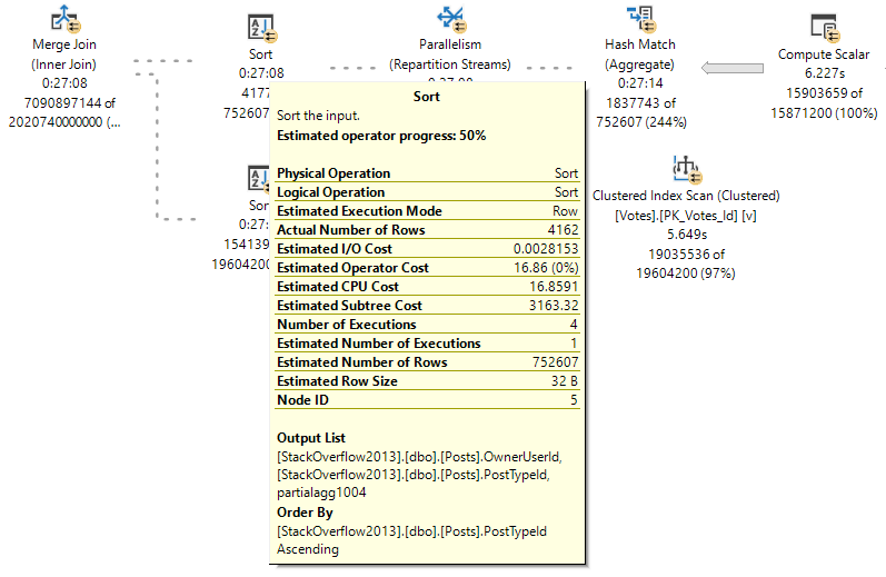
An Adaptive Join Regression In SQL Server

Adaptive joins are a new feature in SQL Server 2017. For adaptive join operators the decision to do a hash or loop join is deferred until enough input rows are counted. You can get an introduction on the topic in this blog post by Joe Sack. Dmitry Pilugin has an excellent post digging into the internals. The rest of this blog post assumes that you know the basics of adaptive joins.

Getting an Adaptive Join


It’s pretty easy to create a query that has an adaptive join in SQL Server 2017. Below I create a CCI with 100k rows and an indexed rowstore table with 400k rows:

DROP TABLE IF EXISTS dbo.MY_FIRST_CCI;

CREATE TABLE dbo.MY_FIRST_CCI (
	FILTER_ID_1 INT NOT NULL,
	FILTER_ID_2 INT NOT NULL,
	FILTER_ID_3 INT NOT NULL,
	JOIN_ID INT NOT NULL,
	INDEX CI CLUSTERED COLUMNSTORE
);

INSERT INTO dbo.MY_FIRST_CCI WITH (TABLOCK)
SELECT TOP (100000)
  t.RN
, t.RN
, t.RN
, t.RN
FROM
(
	SELECT ROW_NUMBER() OVER (ORDER BY (SELECT NULL)) RN
	FROM master..spt_values t1
	CROSS JOIN master..spt_values t2
) t
OPTION (MAXDOP 1);

ALTER TABLE dbo.MY_FIRST_CCI REBUILD WITH (MAXDOP = 1);

CREATE STATISTICS S1 ON dbo.MY_FIRST_CCI (FILTER_ID_1)
WITH FULLSCAN;
CREATE STATISTICS S2 ON dbo.MY_FIRST_CCI (FILTER_ID_2)
WITH FULLSCAN;
CREATE STATISTICS S3 ON dbo.MY_FIRST_CCI (FILTER_ID_3)
WITH FULLSCAN;
CREATE STATISTICS S4 ON dbo.MY_FIRST_CCI (JOIN_ID)
WITH FULLSCAN;

DROP TABLE If exists dbo.SEEK_ME;

CREATE TABLE dbo.SEEK_ME (
	JOIN_ID INT NOT NULL,
	PADDING VARCHAR(2000) NOT NULL,
	PRIMARY KEY (JOIN_ID)
);

INSERT INTO dbo.SEEK_ME WITH (TABLOCK)
SELECT TOP (400000)
  ROW_NUMBER() OVER (ORDER BY (SELECT NULL))
, REPLICATE('Z', 2000)
FROM master..spt_values t1
CROSS JOIN master..spt_values t2

CREATE STATISTICS S1 ON dbo.SEEK_ME (JOIN_ID)
WITH FULLSCAN;

The full scan stats are just there to show that there isn’t any funny business with the stats. The below query gets an adaptive join:

SELECT *
FROM dbo.MY_FIRST_CCI o
INNER JOIN dbo.SEEK_ME i ON o.JOIN_ID = i.JOIN_ID

It’s obvious when it happens in SSMS:

a16_sample_adaptive_join

It’s possible to get an adaptive join with even simpler table definitions. I created the tables this way because they’ll be used for the rest of this post.

Adaptive Threshold Rows


Unlike some other vendors, Microsoft was nice enough to expose the adaptive row threshold in SSMS when looking at estimated or actual plans:

a16_threshold

The adaptive join saves input rows to a temporary structure and acts as a blocking operator until it makes a decision about which type of join to use. In this example, if there are less than 80388.3 rows then the adaptive join will execute as a nested loop join. Otherwise it’ll execute as a hash join.

The adaptive threshold row count can change quite a bit based on the input cardinality estimate. It changes to 22680 rows if I add the following filter that results in a single row cardinality estimate:

WHERE o.FILTER_ID_1 = 1

It was surprising to me to see so much variance for this query. There must be some overhead with doing the adaptive join but I wouldn’t expect the tipping point between a loop and hash join to change so dramatically. I would expect it to be close to a traditional tipping point calculated without adaptive joins.

Traditional Tipping Point


Let’s disable adaptive joins using the 'DISABLE_BATCH_MODE_ADAPTIVE_JOINS' USE HINT and consider how an execution plan would look for this query:

SELECT *
FROM dbo.MY_FIRST_CCI o
INNER JOIN dbo.SEEK_ME i ON o.JOIN_ID = i.JOIN_ID
WHERE o.FILTER_ID_1 BETWEEN @start AND @end
OPTION (
RECOMPILE,
USE HINT('DISABLE_BATCH_MODE_ADAPTIVE_JOINS')
);

We should expect a hash join if the local variables don’t filter out as many rows. Conversely, we should expect a loop join if the local variables on FILTER_ID_1 filter out many rows from the table. There’s a tipping point where the plan will change from a hash join to a loop join if we filter out a single additional row . On my machine, the tipping point is between 48295 and 48296 rows:

a16_fixed_tipping_point.PNG

The estimated costs for the two queries are very close to each other: 74.6842 and 74.6839 optimizer units. However, we saw earlier that the tipping point for an adaptive join on this query can vary between 22680 and 80388.3 rows. This inconsistency means that we can find a query that performs worse with adaptive joins enabled.

The Regression


After some trial and error I found the following query:

SELECT *
FROM dbo.MY_FIRST_CCI o
INNER JOIN dbo.SEEK_ME i ON o.JOIN_ID = i.JOIN_ID
WHERE o.FILTER_ID_1 BETWEEN 1 AND 28000
AND o.FILTER_ID_2 BETWEEN 1 AND 28000
AND o.FILTER_ID_3 BETWEEN 1 AND 28000
ORDER BY (SELECT NULL)
	OFFSET 100001 ROWS FETCH NEXT 1 ROW ONLY
OPTION (MAXDOP 1);

The ORDER BY stuff isn’t important. It’s there just to not send any rows over the network. Here’s the plan:

a16_regression

The query has a cardinality estimate of 10777.7 rows coming out of the MY_FIRST_CCI table. The adaptive join has a tipping point of 27611.6 rows. However, I’ve constructed the table and the filter such that 28000 rows will be sent to the join. SQL Server expects a loop join, but it will instead do a hash join because 28000 > 27611.6. With a warm cache the query takes almost half a second:

CPU time = 469 ms, elapsed time = 481 ms.

If I disable adaptive joins, the query finishes in less than a fifth of a second:

CPU time = 172 ms, elapsed time = 192 ms.

A loop join is a better choice here, but the adaptive row threshold makes the adaptive join pick a hash join.

Final Thoughts


This post contains only a single test query, so it’s no cause for panic. It’s curious that Microsoft made the adaptive join tipping so dependent on cardinality estimates going into the join. I’m unable to figure out the design motivation for doing that. I would expect the other side of the join to be much more important.

Thanks for reading!

Going Further


If this is the kind of SQL Server stuff you love learning about, you’ll love my training. Blog readers get 25% off the Everything Bundle — over 100 hours of performance tuning content. Need hands-on help? I offer consulting engagements from targeted investigations to ongoing retainers. Want a quick sanity check before committing to a full engagement? Schedule a call — no commitment required.