My least favorite tempdb spills are the ones that happen with a large percentage of the memory grant remaining unused. For example, recently I saw tempdb spills with a memory grant of 35 GB but SQL Server reported that only 10 GB of memory was used. Usually this problem can be traced back to suboptimal memory fractions somewhere in a query plan. I suspect that it can also happen with certain types of queries that load data into columnstore tables but haven’t verified that. In the test environment the issue was caused by memory fractions, but these memory fractions were attached to batch mode operators. The rules for batch mode memory fractions certainly appear to be different than those for rowstore memory fractions. I believe that I was able to work out a few of the details for a few simple cases. In some scenarios, plans with multiple batch mode hash joins can ask for significantly more memory than needed. Reducing the memory grant via Resource Governor or a query hint to something more reasonable can lead to unnecessary (and often frustrating) tempdb spills.
What is a Memory Fraction?
There’s very little information out there about memory fractions. I would define them as information in the query plan that can give you clues about each operator’s share of the total query memory grant. This is naturally more complicated for query plans that insert into tables with columnstore indexes but that won’t be covered here. Most references will tell you not to worry about memory fractions or that they aren’t useful most of the time. Out of thousands of queries that I’ve tuned I can only think of a few for which memory fractions were relevant. Sometimes queries spill to tempdb even though SQL Server reports that a lot of query memory was unused. In these situations I generally hope for a poor cardinality estimate which leads to a memory fraction which is too low for the spilling operator. If fixing the cardinality estimate doesn’t prevent the spill then things can get a lot more complicated, assuming that you don’t just give up.
Types of Query Plans
The demos for this blog post all use tables with identical structures and data. The tables are heaps so the plans will only feature hash joins. The most important plan characteristic is how many of the hash tables need to be kept in memory concurrently while the query processor executes the query. This is where memory fractions come in. The query optimizer tries to reuse parts of memory grants as it can. For example, if the hash build for the first join isn’t needed when the third join executes then it’s possible to use the memory grant from the first hash table for the third hash table. Some of the examples below will make this more clear.
The first type of plan has hash joins which can all run concurrently. Memory for the hash tables cannot be reused between operators.
For that query, the MF_DEMO_1 table is the probe side for all of the joins. SQL Server builds all of the hash joins and then rows flow from the probe side through the plan (as long as there aren’t tempdb spills). I will refer to this type of plan as a “concurrent join plan” which is a term that I just made up.
The second type of plan has hash joins which cannot all run concurrently. Pairs of hash tables are active at the same time, but memory grants can be reused between operators.
For that query, the MF_DEMO_1 table is the build side for all of the joins. Each hash table blocks the next one from starting. This means that at most two hash tables need to be kept in memory at the same time. Query memory cannot be reused for joins 1 and 2 but join 3 can reuse memory from join 1 and join 4 can reuse memory from join 2. I will refer to this type of plan as a “nonconcurrent join plan” which is another term that I just made up.
If the above wasn’t clear I recommend running through the demos with live query statistics enabled. It can be very useful to understand how rows flow through a plan. As far as I know, all queries of this type can be implemented with the nonconcurrent pattern but not all queries can be implemented with the concurrent pattern .
Create the Tables
The table definitions for our demos are pretty boring. I’m using a VARCHAR(100) as the join column to blow up memory grants and requirements a bit. All of the tables are heaps and have about 6.5 million rows in them. TARGET_TABLE is used as a dumping ground for the inserts and #ADD_BATCH_MODE is used to switch the hash joins to batch mode as desired. All testing was done on SQL Server 2016 SP1 CU7.
DROP TABLE IF EXISTS MF_DEMO_1;
CREATE TABLE MF_DEMO_1 (
ID VARCHAR(100)
);
INSERT INTO MF_DEMO_1 WITH (TABLOCK)
SELECT 999999999999999 + ROW_NUMBER()
OVER (ORDER BY (SELECT NULL))
FROM master..spt_values t1
CROSS JOIN master..spt_values t2;
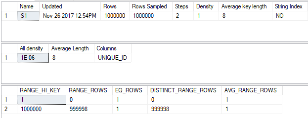
CREATE STATISTICS S1 ON MF_DEMO_1 (ID) WITH FULLSCAN;
DROP TABLE IF EXISTS MF_DEMO_2;
CREATE TABLE MF_DEMO_2 (
ID VARCHAR(100)
);
INSERT INTO MF_DEMO_2 WITH (TABLOCK)
SELECT 999999999999999 + ROW_NUMBER()
OVER (ORDER BY (SELECT NULL))
FROM master..spt_values t1
CROSS JOIN master..spt_values t2;
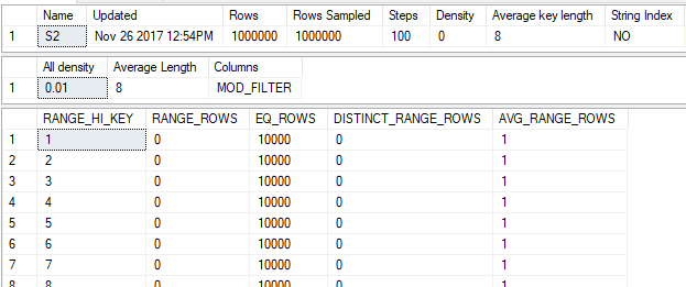
CREATE STATISTICS S2 ON MF_DEMO_2 (ID) WITH FULLSCAN;
DROP TABLE IF EXISTS MF_DEMO_3;
CREATE TABLE MF_DEMO_3 (
ID VARCHAR(100)
);
INSERT INTO MF_DEMO_3 WITH (TABLOCK)
SELECT 999999999999999 + ROW_NUMBER()
OVER (ORDER BY (SELECT NULL))
FROM master..spt_values t1
CROSS JOIN master..spt_values t2;
CREATE STATISTICS S3 ON MF_DEMO_3 (ID) WITH FULLSCAN;
DROP TABLE IF EXISTS MF_DEMO_4;
CREATE TABLE MF_DEMO_4 (
ID VARCHAR(100)
);
INSERT INTO MF_DEMO_4 WITH (TABLOCK)
SELECT 999999999999999 + ROW_NUMBER()
OVER (ORDER BY (SELECT NULL))
FROM master..spt_values t1
CROSS JOIN master..spt_values t2;
CREATE STATISTICS S4 ON MF_DEMO_4 (ID) WITH FULLSCAN;
DROP TABLE IF EXISTS MF_DEMO_5;
CREATE TABLE MF_DEMO_5 (
ID VARCHAR(100)
);
INSERT INTO MF_DEMO_5 WITH (TABLOCK)
SELECT 999999999999999 + ROW_NUMBER()
OVER (ORDER BY (SELECT NULL))
FROM master..spt_values t1
CROSS JOIN master..spt_values t2;
CREATE STATISTICS S5 ON MF_DEMO_5 (ID) WITH FULLSCAN;
CREATE TABLE #ADD_BATCH_MODE (I INT, INDEX CCI CLUSTERED COLUMNSTORE);
DROP TABLE IF EXISTS TARGET_TABLE;
CREATE TABLE TARGET_TABLE (ID VARCHAR(100));
Row Mode Memory Fractions For Concurrent Join Plans
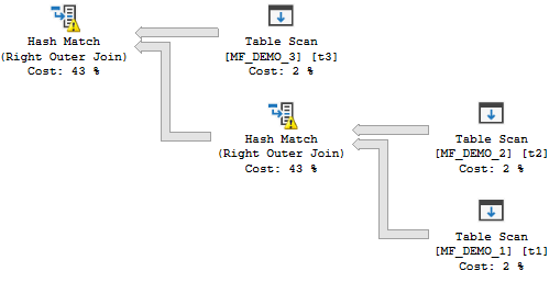
The following query results in a concurrent join plan with row mode hash joins:
INSERT INTO TARGET_TABLE WITH (TABLOCK)
SELECT t1.ID
FROM MF_DEMO_3 t3
RIGHT OUTER JOIN MF_DEMO_2 t2
RIGHT OUTER JOIN MF_DEMO_1 t1
ON t1.ID = t2.ID
ON t1.ID = t3.ID
OPTION (FORCE ORDER, MAXDOP 1);
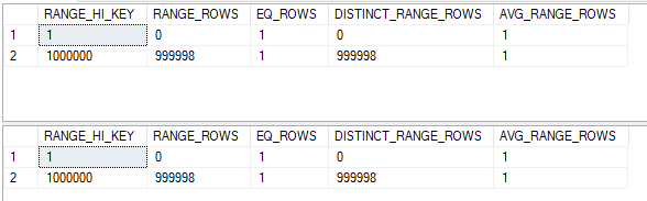
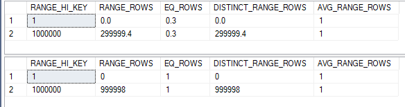
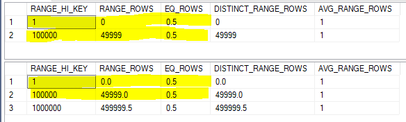
The desired memory grant is 2860640 KB. The memory fractions for both join operators have an input of 0.5 and an output of 0.5. This is exactly as expected. The hash tables can both start at the same time and cannot reuse memory, so each operator gets 50% of the query memory grant for the plan. Adding a third join to the plan increases the query memory grant to 4290960 KB.
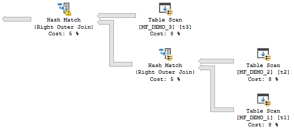
INSERT INTO TARGET_TABLE WITH (TABLOCK)
SELECT t1.ID
FROM MF_DEMO_4 t4
RIGHT OUTER JOIN MF_DEMO_3 t3
RIGHT OUTER JOIN MF_DEMO_2 t2
RIGHT OUTER JOIN MF_DEMO_1 t1
ON t1.ID = t2.ID
ON t1.ID = t3.ID
ON t1.ID = t4.ID
OPTION (FORCE ORDER, MAXDOP 1);
Again, this seems very reasonable. SQL Server now tries to builds three hash tables in memory at the same time. The memory fractions for each operator have fallen to 0.3333333. Each operator gets a third of the query memory grant.
Row Mode Memory Fractions For Nonconcurrent Join Plans
The following query results in a nonconcurrent join plan with row mode hash joins:
INSERT INTO TARGET_TABLE WITH (TABLOCK)
SELECT t1.ID
FROM MF_DEMO_1 t1
INNER JOIN MF_DEMO_2 t2 ON t1.ID = t2.ID
INNER JOIN MF_DEMO_3 t3 ON t2.ID = t3.ID
INNER JOIN MF_DEMO_4 t4 ON t3.ID = t4.ID
OPTION (MAXDOP 1, FORCE ORDER);
The query plan was uploaded here. I recommend downloading the all of the plans referenced in this blost post if you’re interested in them so you can see all of the details.
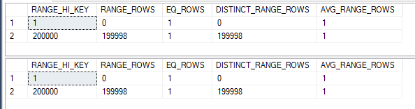
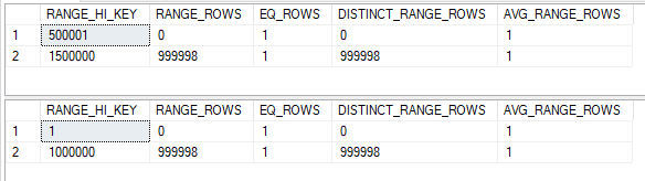
Here are the memory fractions for the rightmost join (node 3):
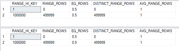
Memory Fractions Input: 1, Memory Fractions Output: 0.476174
here are the memory fractions for the middle join (node 2):
Memory Fractions Input: 0.523826, Memory Fractions Output: 0.5
and here are the memory fractions for the leftmost join (node 1):
Memory Fractions Input: 0.5, Memory Fractions Output: 1
What do all of those numbers mean? The rightmost join builds its hash table first and starts with all query memory available to it. However, the output fraction is 0.476174. That means that the hash table can only use up to 47.6% of the query memory granted to the plan. The middle join is able to use up to 50% (the minimum of the input and output fractions for the node) of the memory granted to the plan. Note that 0.476174 + 0.523826 = 1.0. The last join to start executing is also able to use up to 50% of the granted memory. That join is the last operator that uses memory in the plan so the output fraction is 1.0. Memory grant reuse allows the plan to use up to 147.6% of the memory grant over the lifetime of the query execution. Without memory grant reuse each operator wouldn’t be able to use as much memory.
Removing one of the joins results in the desired query memory grant dropping from 3146704 KB to 3003672 KB. This is a significantly less drop than the other query. The smaller decrease is expected because the third join that we added can reuse the memory grant from the first. As more joins are added to a nonconcurrent plan the desired memory grant grows at a much slower rate than the memory grant for the concurrent join plan.
Batch Mode Memory Fractions For Concurrent Join Plans
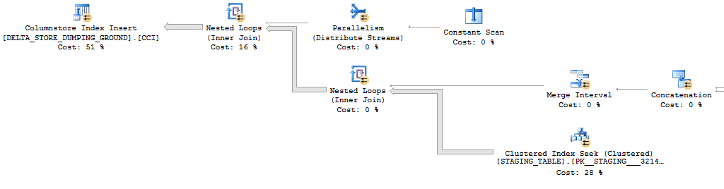
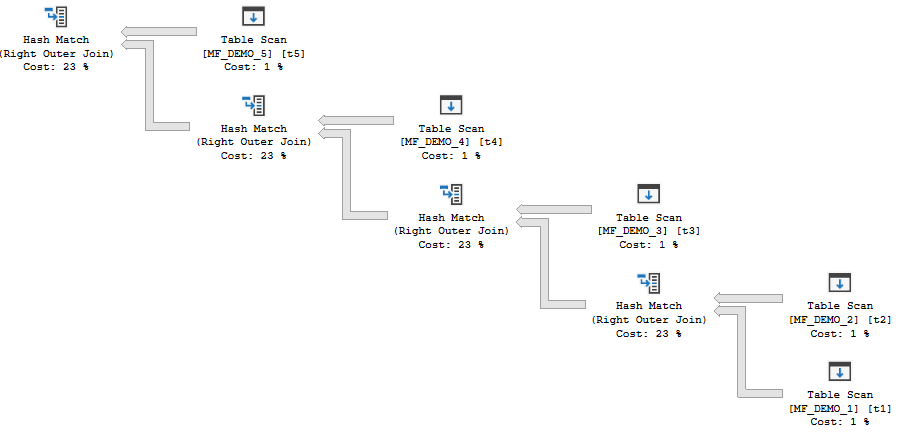
The query plan for the next query is somewhat dependent on hardware. On my machine I had to let it run in parallel to get batch mode hash joins:
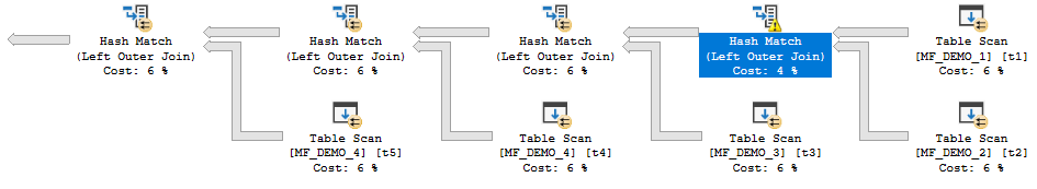
INSERT INTO TARGET_TABLE WITH (TABLOCK)
SELECT t1.ID
FROM MF_DEMO_5 t5
RIGHT OUTER JOIN MF_DEMO_4 t4
RIGHT OUTER JOIN MF_DEMO_3 t3
RIGHT OUTER JOIN MF_DEMO_2 t2
RIGHT OUTER JOIN MF_DEMO_1 t1
LEFT OUTER JOIN #ADD_BATCH_MODE ON 1 = 0
ON t1.ID = t2.ID
ON t1.ID = t3.ID
ON t1.ID = t4.ID
ON t1.ID = t5.ID
OPTION (FORCE ORDER, MAXDOP 4);
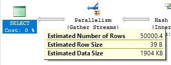
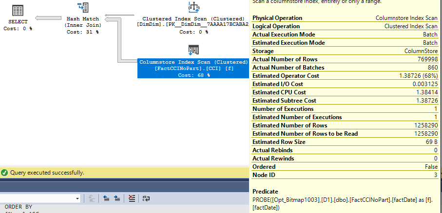
The estimated plan is here. It’s easy to tell if the query is using batch mode joins because the joins are run in parallel but there are no repartition stream operators.
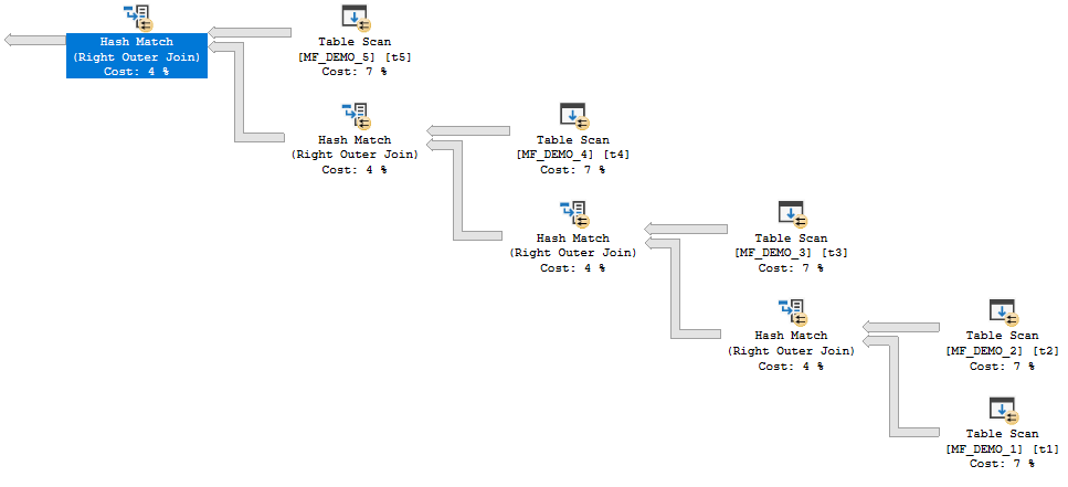
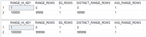
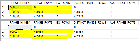
SQL Server is not able to reuse memory grants for this query. SQL Server tries to build all of the hash tables in memory before probe side is processed. However, the memory fractions are different from before: 0.25, 0.5, 0.75, and 1.0. These memory fractions do not make sense if interpreted in the same way as before. How can the final hash join in the plan have an input memory fraction of 1.0?
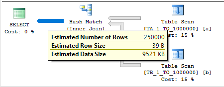
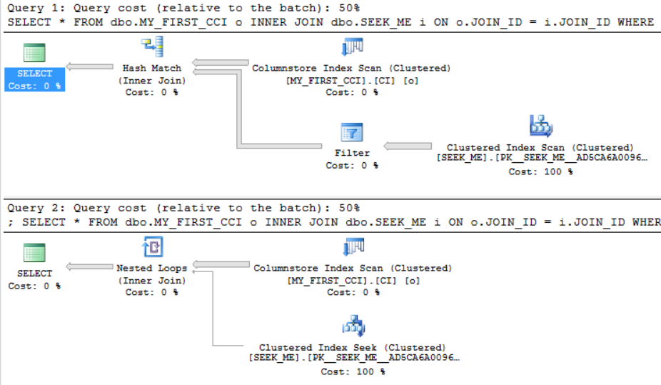
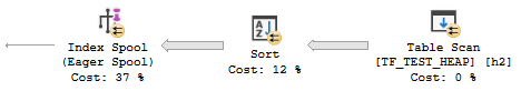
It’s unclear what the memory fractions are supposed to mean here, but there is one observable difference compared to the row mode plan. In the row mode equivalent plan SQL Server divides the memory evenly between operators. For our very simple test plan this means that all of the hash joins will spill to tempdb or none of them will spill. Reducing a MAX_GRANT_PERCENT hint from the right value by 1% results in two spills:
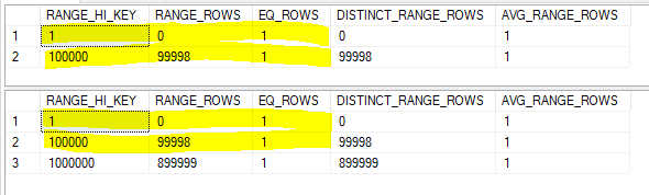
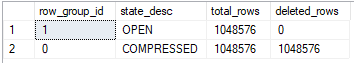
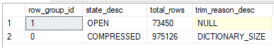
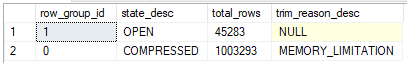
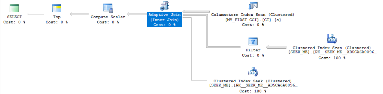
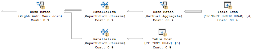
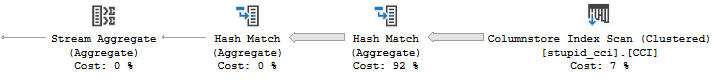
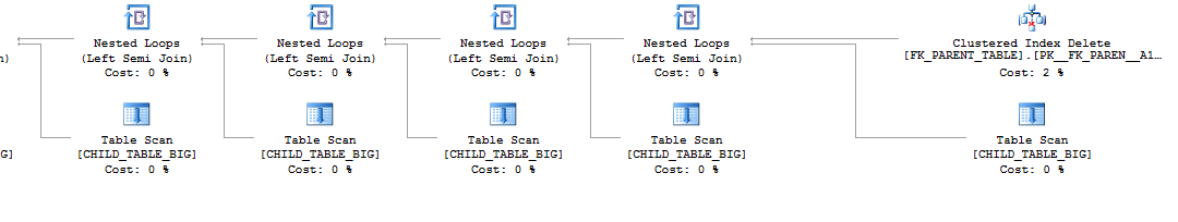
Both operators spilled because memory was divided evenly and there wasn’t enough memory to hold both hash tables in memory. However, with batch mode hash joins we can get plans like the following:
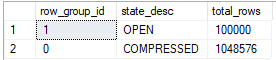
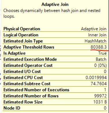
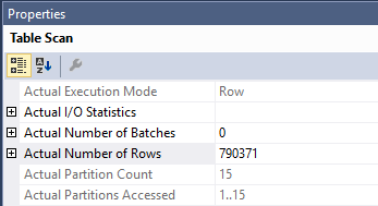
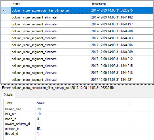
How is it possible that one join spills but the other doesn’t? It is only possible if memory isn’t divided evenly. It appears that memory is used as needed in some situations. Unfortunately, the actual plan for batch mode operators doesn’t give us a lot of spill information like it does for row mode. There’s a debug channel extended event query_execution_batch_hash_join_spilled that can give us some clues. 657920 KB of memory was granted for a two batch mode hash join query. For the operator that spilled, only 44852457 bytes were written to memory on the build side. That’s about 43800 KB, which is significantly less than half of available query memory.
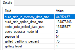
We can’t conclude that exactly 44852457 bytes of memory were granted to the operator. However, it should be somewhat close. In conclusion, for these types of queries it isn’t clear what the memory grant fractions are supposed to mean. SQL Server is able to exceed them in some cases. It’s possible to see 0 bytes of memory used for the build side in the extended event. I believe that this is the bad type of memory reuse as opposed to the good kind.
Batch Mode Memory Fractions For Nonconcurrent Join Plans
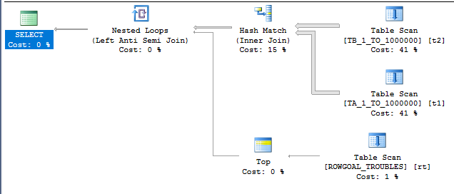
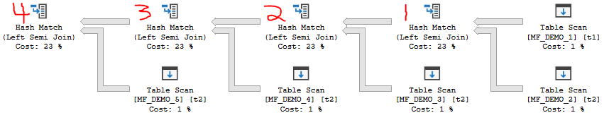
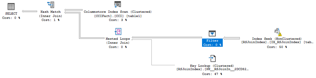
The following query results in a nonconcurrent batch mode hash join plan on my machine:
INSERT INTO TARGET_TABLE WITH (TABLOCK)
SELECT t1.ID
FROM MF_DEMO_1 t1
LEFT OUTER JOIN #ADD_BATCH_MODE On 1 = 0
WHERE EXISTS (
	SELECT 1
	FROM MF_DEMO_2 t2 WHERE t1.ID = t2.ID
) AND EXISTS (
	SELECT 1
	FROM MF_DEMO_3 t3 WHERE t1.ID = t3.ID
) AND EXISTS (
	SELECT 1
	FROM MF_DEMO_4 t4 WHERE t1.ID = t4.ID
) AND EXISTS (
	SELECT 1
	FROM MF_DEMO_5 t5 WHERE t1.ID = t5.ID
) OPTION (MAXDOP 4, FORCE ORDER);
As far as I know there’s nothing special about the semijoins. I used them to keep the estimated row size as consistent as possible. The behavior detailed below can be observed with normal joins as well.
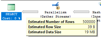
Here is the estimated query plan. The same memory fraction pattern of 0.25, 0.50, 0.75, and 1.00 can be found in this query. Based on the query’s structure, memory grant reuse should be allowed between operators. Alarmingly, this query has the same desired memory grant as one with four concurrent joins. The desired memory grant changes significantly as tables are added or removed. This is a big change in behavior compared to row mode batch joins.
As far as I can tell, memory grant reuse can happen in plans like this with batch mode hash joins. Removing or adding joins results in very small adjustments in maximum memory used during query execution. Still, it seems as if the query optimizer is assuming that memory cannot be reused. With this query pattern, the first operator to run does not have access more memory implied by the memory fraction. In fact, it has access to less memory implied by the memory fraction.
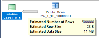
Running the query without any memory grant hints results in no tempdb spills and a maximum memory use of 647168 KB. Restricting the memory grant to 2 GB results in a tempdb spill for the rightmost operator. This is unexpected. 500000 KB of memory should be more than enough memory to avoid a spill. As before, the only way I could find to investigate this further was to use the query_execution_batch_hash_join_spilled extended event and to force tempdb spills using the MAX_GRANT_PERCENT query hint.
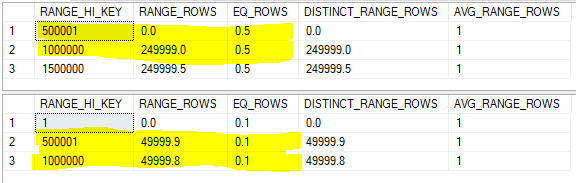
A good amount of testing suggested that the available memory per operator is the input memory fraction for that operator divided by the sum of all output memory fractions. The rightmost operator only gets 0.25 / (0.25 + 0.5 + 0.75 + 1.0) = 10% of the memory granted to the query, the next operator gets 20%, the next operator gets 30%, and the final operator gets 40%. The situation gets worse as more joins are added to the query. Keep in mind that we aren’t doing anything tricky with cardinality estimates or data types which would result in skewed estimates. The query optimizer seems to recognize that each join will require the same amount of memory for each hash join, but it doesn’t make the same minimum amount available for each operator. That’s what is so puzzling.
The preceding paragraph seems to contradict the idea that memory grant reuse is possible for these plan shapes. Perhaps for these simple plans memory grant reuse is possible but it cannot go above 100% like we saw in the row mode plan. This could still be helpful in that the query could steal less memory from the buffer pool, but it’s certainly not as helpful in avoiding spills as the behavior we get with the row mode plan. Under the assumption the total memory grants seem a bit more reasonable, although it’s hard not to object as to how SQL Server is distributing the memory to each operator.
We can avoid the spill by giving SQL Server the memory that it required, but this is undesirable if multiple concurrent queries are running. I’ve often observed higher than expected memory grants for queries with batch mode hash joins. An assumption that query memory reuse will not be available for batch mode hash joins can explain part of what I’ve observed. If memory grants are left unchecked, applications may see decreased possible concurrency due to RESOURCE_SEMAPHORE waits. Lowering memory grants through any available method can result in unnecessary (based on total memory granted) tempdb spills. It’s easy to get stuck between a rock and a hard place.
Batch Mode Workarounds
There is some hope for nonconcurrent batch mode hash join plans. SQL Server 2017 introduces adaptive memory feedback for these operators. I imagine that functionality is a poor fit for ETL queries which may process dramatically different amounts of data each day, so I can’t view it as a complete solution. It certainly doesn’t help us on SQL Server 2016. Are there workarounds to prevent spills without requiring excessive memory grants? Yes, but they are very ugly and I can only imagine using them when truly needed during something like an ETL process.
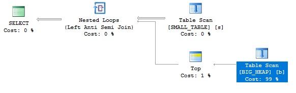
Consider the following query:
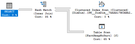
INSERT INTO TARGET_TABLE WITH (TABLOCK)
SELECT t1.ID
FROM MF_DEMO_1 t1
LEFT OUTER JOIN MF_DEMO_2 t2 ON t2.ID = t1.ID
LEFT OUTER JOIN MF_DEMO_3 t3 ON t3.ID = t2.ID
LEFT OUTER JOIN MF_DEMO_4 t4 ON t4.ID = t3.ID
LEFT OUTER JOIN MF_DEMO_4 t5 ON t5.ID = t4.ID
LEFT OUTER JOIN #ADD_BATCH_MODE ON 1 = 0
OPTION (FORCE ORDER, MAXDOP 4, MAX_GRANT_PERCENT = 60);
On my machine, the memory hint results in a memory grant of 2193072 KB. The rightmost join spills even when only a maximum of 1232896 KB of memory is used during query execution:
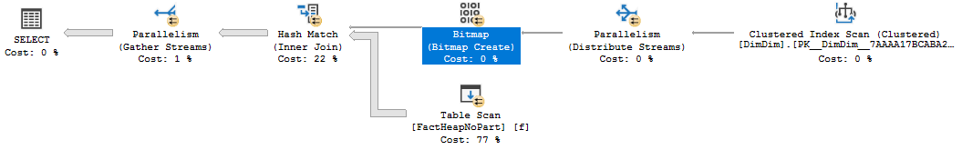
One way to avoid the spill is to shift the memory fractions in our favor. Ideally SQL Server would think that the rightmost join would need much more memory for its hash table than the other joins. If we can add an always NULL column with a large data type that is only needed for the first hash table, that might do the trick. The query syntax below isn’t guaranteed to get the plan that we want but it seems to work in this case:
ALTER TABLE MF_DEMO_1 ADD DUMMY_COLUMN_V4000 VARCHAR(4000) NULL;
ALTER TABLE MF_DEMO_2 ADD DUMMY_COLUMN_V10 VARCHAR(10) NULL;

INSERT INTO TARGET_TABLE WITH (TABLOCK)
SELECT t1.ID
FROM MF_DEMO_1 t1
LEFT OUTER JOIN MF_DEMO_2 t2 ON t2.ID = t1.ID
LEFT OUTER JOIN MF_DEMO_3 t3 ON t3.ID = t2.ID
LEFT OUTER JOIN MF_DEMO_4 t4 ON t4.ID = t3.ID
LEFT OUTER JOIN MF_DEMO_4 t5 ON t5.ID = t4.ID
LEFT OUTER JOIN #ADD_BATCH_MODE ON 1 = 0
WHERE (t1.DUMMY_COLUMN_V4000 IS NULL OR t2.DUMMY_COLUMN_V10 IS NULL)
OPTION (FORCE ORDER, MAXDOP 4, MAX_GRANT_PERCENT = 32);
An actual plan was uploaded here. The query no longer spills even though the memory grant was cut to 1225960 KB. The memory fractions are now 0.82053, 0.878593, 0.936655, and 1. The change was caused by the increase in estimated row size for the rightmost join: 2029 bytes. That row size is reduced to 45 bytes after the filter is applied, which won’t filter out any rows because both columns are always NULL. The FORCE ORDER hint is essential to get this plan shape. It’s very unnatural otherwise.
If the same rules are followed as before, the rightmost join should get 22.5% of the available query memory grant now. This is enough to avoid the spill to tempdb.
Final Thoughts
I understand that the formulas for memory fractions need to account for an arbitrary combination of row mode and batch mode operators in a query plan. However, it is disappointing that the available information for memory fractions for batch mode operators is so confusing, some queries with batch mode hash joins ask for way more memory than they need, and some queries needlessly spill to tempdb without using close to their full memory grant. Batch mode adaptive memory grant feedback can offer some relief in SQL Server 2017, but why not expect good plans the first time as long as we’re giving the query optimizer good information?
Thanks for reading!
Going Further
If this is the kind of SQL Server stuff you love learning about, you’ll love my training. I’m offering a 75% discount to my blog readers if you click from here. I’m also available for consulting if you just don’t have time for that and need to solve performance problems quickly.

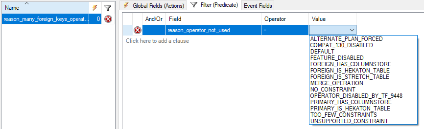 Is trace flag 9448 a previously unknown (to the community) trace flag? Sure looks like it:
 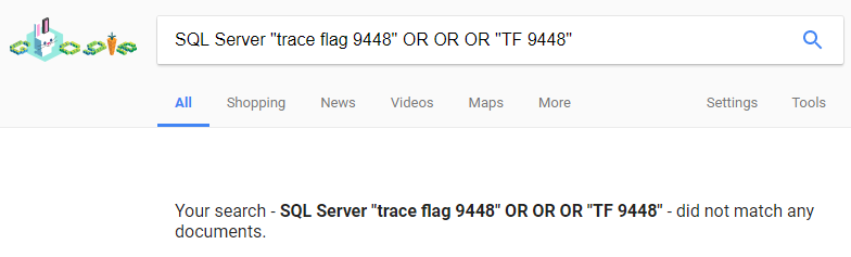 Not a very useful one, but I can cross “discover a trace flag” off my bucket list. I searched around a bit in